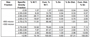
As may be seen from the table, a separation at S.G. 2.75 would result in a float product of 68.5% of the weight contain 3.8% of the tin of that size fraction.  Laboratory separations in heavy liquids are “ideal” – all the sinks should report to the sinks and all the floats to the floats. In industrial applications heavy media is used (rather than the organic heavy liquids) and inefficiencies in the separation are seen (i.e. sinks misreporting into floats and vice versa). This is because particles with the same or near S.G. as that of the media have an equal chance of reporting to either fraction. The efficiency of separation depends on the ability to separate material of s.G. close to that of the medium. This can be represented by a Tromp or Partition curve, which relates to the partition coefficient (i.e. the percentage of feed material of a particular S.G. which reports to the sinks (or floats) product plotted against S.G.).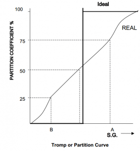 

The ideal (heavy liquid) separation shows that all particles heavier than the separating
density sink, and all those that are lighter, float. The error of separation (known as the Ecart probable – Ep) is defined: Ep = (A – B)/2

As can be seen the lower the Ep the more idealised is the separation. An ideal separation
has an Ep of 0.0, while most practical Ep’s are in the range 0.02-0.08. (Full details of the
construction of Tromp curves are given in Wills (1) pgs 267-274).

Testwork of this type can therefore tell:

• The applicability of preconcentration to a particular ore, and also estimates of actual plant performance.
• The efficiency of H.M.S. units in operation.

The resulting Washability Curves…