The calculation of open pit operations’ capacities has been the subject of many studies using computer simulations. The common problems of simulation are that if one desires a realistic picture of an operation the programming work becomes long and expensive and that the program requires a large computer and long time to run.

The method includes the main parameters of the operation:

1. numbers, sizes and operational availabilities of trucks, shovels and dumping point,
2. distribution of the production over shovels,
3. trucks loading, travel (loaded and empty) and dumping times as well as their variabilities,
4. shift’s composition.

Trucks’ waiting times

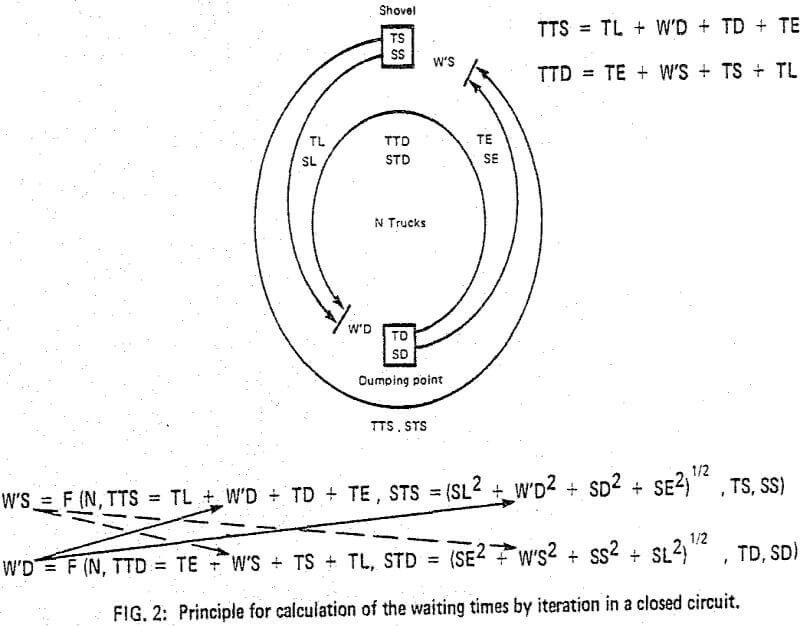
The trucks in a circuit consisting of a shovel, haulage roads for loaded and empty travel and a dumping point will due to their number and the variabilities of loading, loaded and empty travel and dumping times occasionally queue up at the shovel and the dumping point and incur waiting times. These increase with the number of trucks in the circuit and become a substantial part of the trucks’ cycle time, thus limiting the capacity of the system.

During normal operation the trucks’ waiting time will some time after the start of operation attain the level of stationary waiting time which is a function of

1. the number of trucks in the circuit,
2. the average loading time and its standard deviation for trucks at the shovel,
3. the average dumping time and its standard deviation for trucks at the dumping point and
4. the average loaded and empty travel times and their standard deviations for the trucks between the shovel and the dumping point and vice versa.

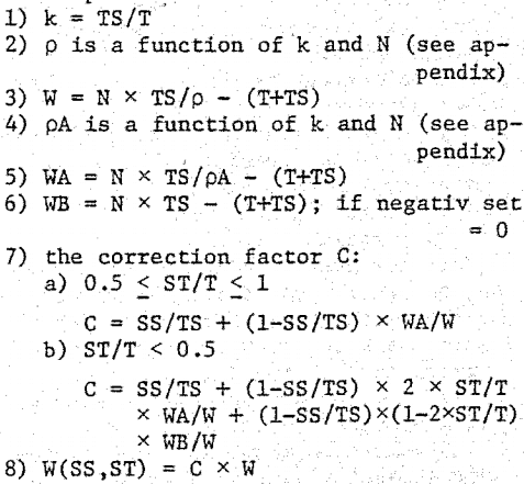
Symbols used:
TS: the average service time
SS: the standard deviation of TS
T: the average return time
ST: the standard deviation of T
N: the number of trucks in the circuit
p: the utilisation of the service station when both TS and T are negative exponentially distributed
W: the average waiting time ahead of the service station in this case
pA: the utilisation of the service station when the return time is negative exponentially distributed and the service time is constant
WA: the average waiting time ahead of the service station in this case
WB: the waiting time ahead of the service station when both return time and service times are constant.
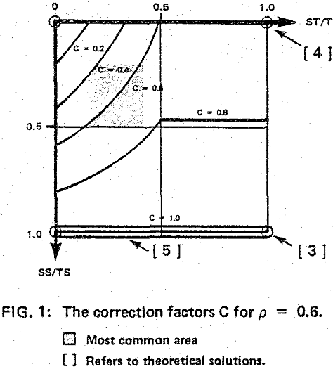
W(SS,ST): the waiting time ahead of the service station when the return time has the standard deviation ST and the service time the standard deviation SS
C: the correction factor

Basic procedure:

Activity times and their standard deviations

These may be obtained by time studies and must include the total occupation by the trucks of the loading position: the actual loading time as well as the times required for maneuvering the truck in and out from the shovel. A time study will also allow that the shovel executes other tanks than actual lending both while a truck is in the loading position and while the loading position is empty. These tanks include such things as cleaning the front, moving a boulder, moving the cable, making a shift etc. If they are of short duration (<½ cycle) they will not cause all the trucks to accumulate at the shovel.

Loaded and empty travel times and their standard deviations are found by time studies. It Is convenient to divide the haulage road into segments according to gradients and lengths and compose the total travel times between a particular shovel location and the dumping point from these. It should be observed that travel times are seasonally variable.

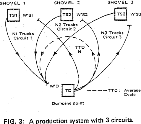
Distribution of shovels and trucks

The shovels are distributed according to target production from the various areas. The trucks are distributed according to target production from the various areas and the related cycle times. The distribution of shovels and trucks results most probably in fractions of shovels and trucks. This can be remedied in two ways – either by choosing integer numbers of shovels and trucks pr shovel over fractions of shift – or by keeping computationally fractions of shovels and trucks, which is possible with the described procedure. The difference between the two methods is not important except in extreme cases.

On the results of a calculation related to an operation with 3 shovels with an operational availability of 75%, various numbers of trucks with an operational availability of 65% and a dumping point with 100% availability. The availability frequency functions have been established assuming the binomial law. The average loading time pr truck is 4.5 min. with standard deviation 1.35 min. The average dumping time pr truck is 1.0 min. with standard deviation 0.3 min. The sum of loaded and empty travel is 12.5 min. with standard deviation 3.75 min. for all 3 shovel locations. The length of the shift is 480 min. with 3 medium length interruptions of each 30 min’s duration.

The estimate of costs can be made by including wages, ownership and costs per ton and ton x mile for energy and maintenance in the calculation. The operational availabilities pr shift were obtained from production reports. It is, however, possible to go one step further and produce the availability frequency functions directly from the parameters of the repair shop for trucks and the repair organization for shovels: