
Table of Contents
Parameters Provided by DPG Research & Development Division
Once the process route and correct Solvent Extraction Equipment type have been decided, the following are the basic design parameters that R & D can provide:
- Reagent and Diluent choice and composition. The composition of the organic phase and of the aqueous input streams enable the isotherm to be determined.
- Equilibrium Isotherm, Stage Efficiencies, Number of stages. Using single stage efficiencies the equilibrium isotherm is converted into the pseudo-equilibrium isotherm and the number of stages predicted using the McCabe Thiele construction.
- Solution Compositions for Mass Balance. These will have been determined by the McCabe-Thiele construction performed above.
- Mixer Residence Time for given impeller type. This is dependent on the kinetics of the mass transfer between phases. The mixer residence time together with the organic: aqueous operating ratio fixes the mixer dimensions according to the formula given in section 3. For typical values for copper systems of this and other parameters see the comparison table.
- Organic/Aqueous operating ratio. The operating O/A ratio is the volume flow ratio of total organic and total aqueous streams entering the mixer box. It will normally be in the region of 1:1 so as to minimise entrainment losses in streams having the settler.
- Settler specific Flowrate. The specific flowrate figure determines the cross-sectional area of the settler. Length-width ratio is approximately 2:1 to 3:1.
- Dispersion Bed Depth. This is related to the settler specific flowrate, and determined entrainment and weir height settings.
For typical values for these parameters see the comparison table for copper SX plants.
R and D Division will also provide assistance with the guarantee statements on entrainments, extraction efficiencies, overall recovery and methods of test for the guarantee run.
Isotherm Prediction from CUAD Curve
The CUAD curve
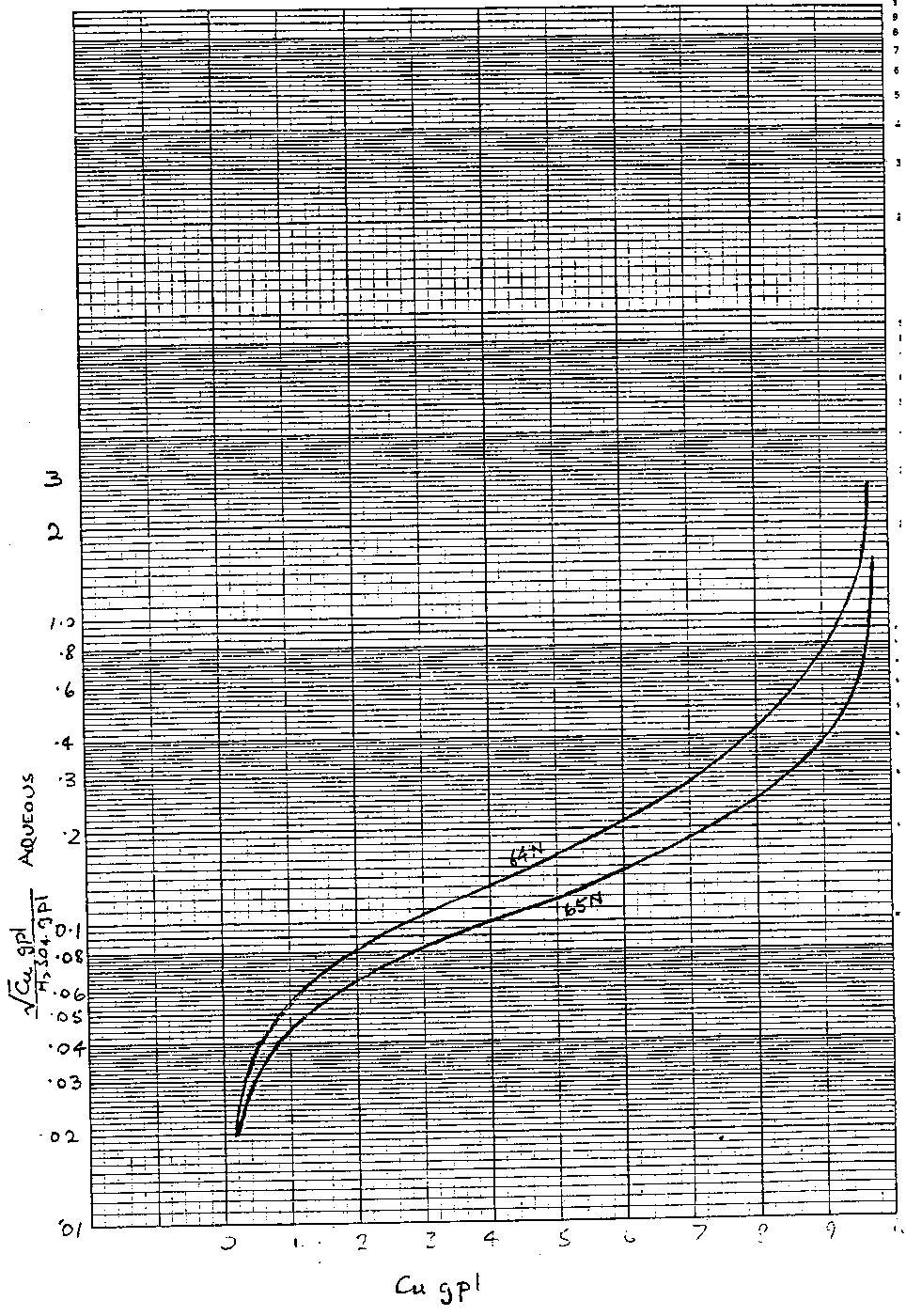
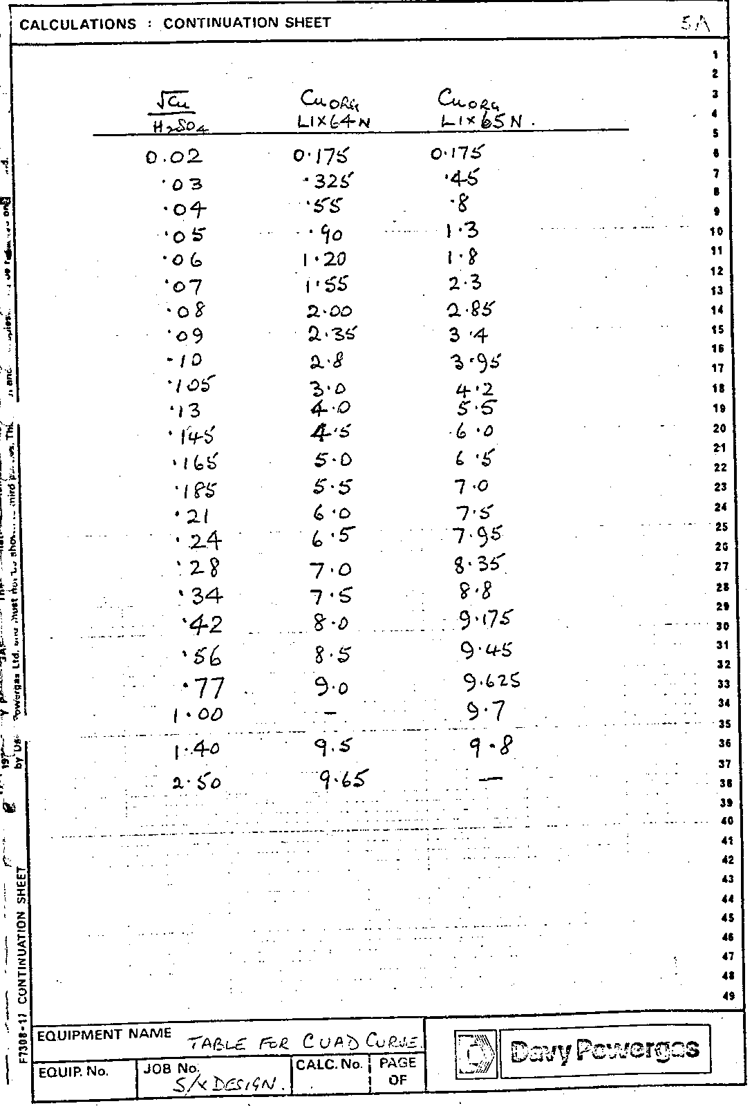
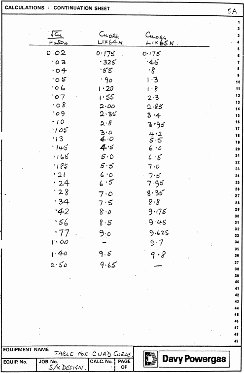
The CUAD curve is a summary of the equilibrium distribution data of acidic copper sulphate solutions in contact with loaded organic solutions. The curves (fig. I ) are drawn for 40% v/v solutions of LIX64N and LIX65N, at t °C, and must be scaled down for other compositions of v% by multiplying the horizontal axis by v/40.
The CUAD curve is a log-linear plot of the square root of the aqueous copper concentration divided by the aqueous sulphuric acid concentration, (( [Cu] )0.5/ [H2SO4 )AQ versus the copper concentration in the organic phase, ([Cu])ORG. All concentrations are expressed in grams per litre.
Prediction of Extraction Isotherm
The isotherm is a plot of the distribution of copper between the two phases at equilibrium. The Extraction Isotherm can be predicted from the CUAD curve if the reagent and concentration are known and also if the pregnant liquor concentration is known.
Readings from the CUAD curve give a set of pairs of coordinates {x,y} where x = [Cu]ORG and Y = (√[Cu] [H2SO4]) AQ.
The original pregnant liquor has composition Co gpl of copper and ac gpl of sulphuric acid. Now, for every mole of copper that is transferred into the organic one mole of sulphuric acid is formed in the aqueous phase (Cu2+ + 2HR ↔ CuR2 + 2H+)
After some copper has been extracted into the organic phase the new aqueous copper concentration is c gpl. Then the new sulphuric acid concentration is ao + 98.08/63.54 (co – c) gpl.
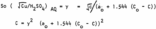
Hence C using the quadratic formula, and rejecting the impossible root.
(for ax² + bx+ c = 0 x= (-b ± √b² – 4ac/2a)
The extraction isotherm is now drawn by plotting x against c. It is normal to plot the aqueous copper concentration on the horizontal axis.
Prediction of Strip Isotherm
The spent electrolyte, or strip liquor, will have composition ao gpl of sulphuric acid and Co gpl of copper. The isotherm is drawn as above (NB. the group (Co – C) will be negative as the copper concentration in the electrolyte is rising).
Interpretation of Equilibrium Isotherms
The method is designed to enable plant operation under specified conditions to be defined in terms of raffinate copper concentration and overall O/A ratio in the strip section. This is achieved by consideration of the copper contents of the loaded and stripped organic streams.
The specified conditions are:
1. Extraction Section
A. Aqueous feed
Cu 2+ gpl, Fe 3+ gpl pH (other impurities gpl)
B. Organic feed
% active solvent v/v in diluent
2. Strip Section
A. Spent electrolyte composition
Cu 2+ gpl, Fe 3+ gpl, free H2SO4 gpl
B. Advance electrolyte composition
Cu 2+ gpl, Fe 3+ gpl, free H2SO4 gpl
Interpretation of the Equilibrium Isotherms
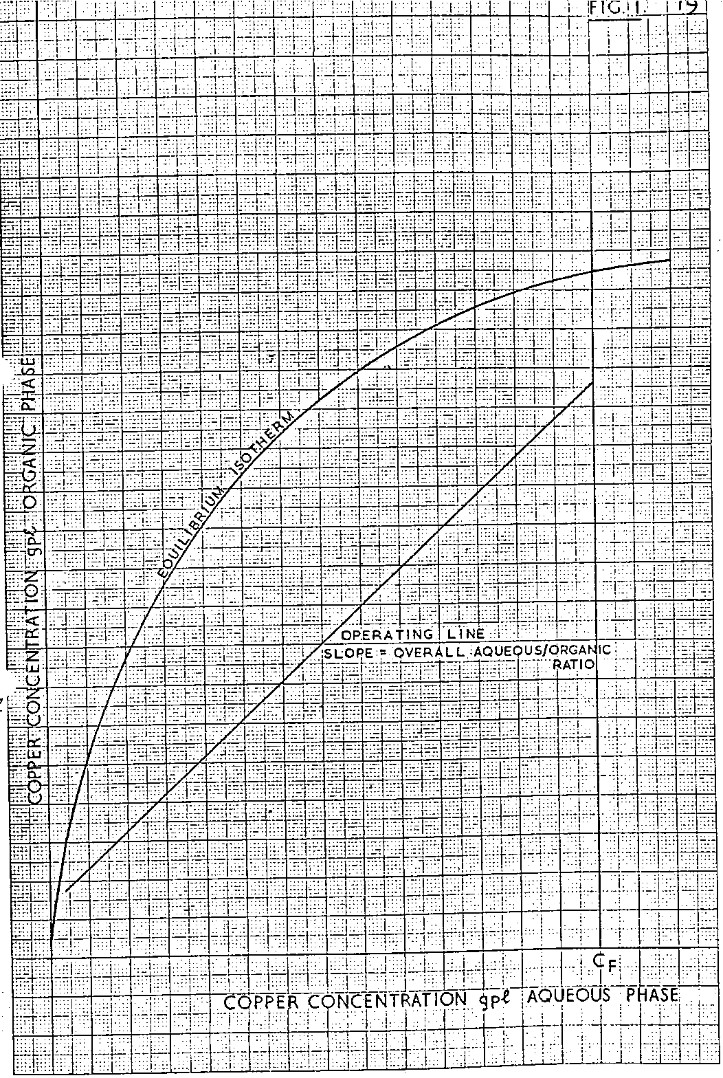
Consider the typical LIX/Cu 2+ extraction and strip equilibrium lines shown diagrammatically plotted on the same axes in Fig 1, where CF represents the aqueous feed copper concentration, C SE the spent electrolyte and C AE, the advance electrolyte copper concentrations.
As a result of inefficiencies which occur in any real system, pseudo equilibrium lines are used in the calculation and these are located by multiplying the equilibrium organic phase copper contents at a variety of points along the equilibrium line by 0.875 for the extraction curve and by 1.143 for the stripping curve and plotting these new values with the corresponding aqueous phase values. These factors were chosen based on previous experience.
The plotting of the extraction and strip isotherms on the same graph is not mandatory, separate plots can also be used.
The determination of the number of stages required to achieve a desired raffinate can now be carried out as follows.
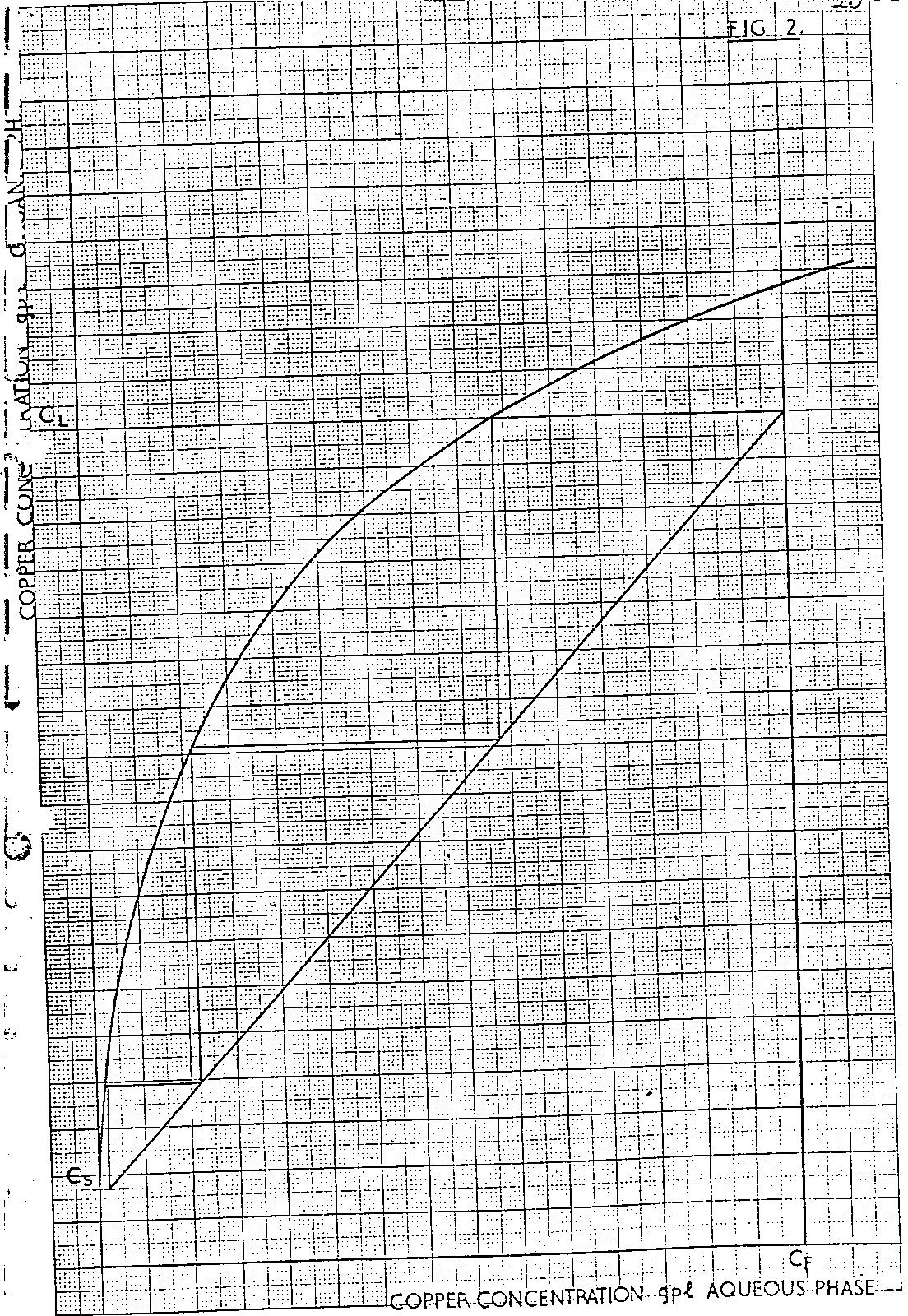
Consider Fig 2. The expected stripped organic copper content C SO is fixed from consideration of the pseudo equilibrium strip line and spent electrolyte copper concentration. Extrapolation of this value to the vertical extrapolation of the spent electrolyte copper content C SE, gives point, A, while intersection with the pseudo strip equilibrium line gives point B.
A 2 stage strip section can now be simulated using the following construction technique.
From the intersection of the copper concentration of the advance electrolyte, C AE with the strip pseudo equilibrium line, point C, draw a horizontal line to intersect with the vertical extrapolation of point B at point D. Then draw a straight line through points A and D to intersect with the copper concentration of the advance electrolyte C AE at point E.
Two stage strip system is now defined, as the horizontal extrapolation of point E gives the loaded organic copper content, C LO , entering the strip section. The overall O/A ratio in the strip section therefore equals
The extraction section can now be defined by constructing the extraction operating line between points O and F, the former being the intersection of the CR and C SO values and the latter being the intersection of the C LO and C F values. Stepping off between this operating line and the pseudo equilibrium line will indicate the number of extraction stages required to achieve the necessary raffinate, although it is unlikely that an exact number of stages will result. However, by changes in raffinate copper concentrations, slope of the extraction section operating line and/or reagent concentration made as a result of results obtained, it is possible, by successive calculation, to determine the exact number of stages required to achieve a given raffinate.
The stimulation of a single strip system is straightforward and can be readily deduced from the above description. Thus, in this case the horizontal extrapolation of point C, the intersection of the advance electrolyte copper concentration C AE and the strip pseudo equilibrium line, gives the stripped organic copper concentration C SO, while the loaded organic copper concentration C LO is obtained
by drawing a straight line of arbitrary chosen slope from the intersection of the C SO and C SE values to intersect the C AE value.
The slope of the line is chosen so that the C LO value produced is within the normal range of percentage of maximum loaded values used in LIX systems, i.e. 50-70% for LIX 64N and LIX 65N.
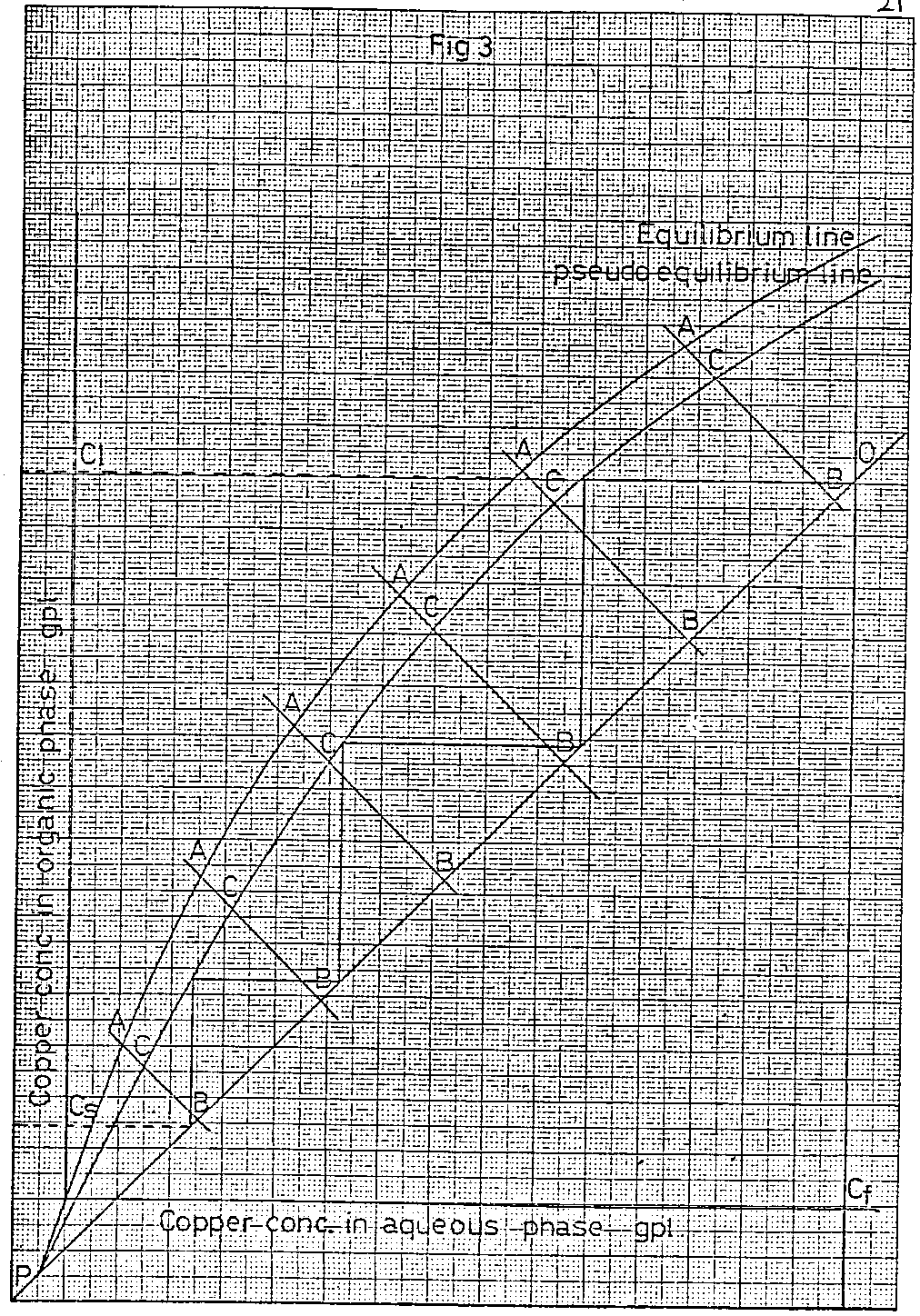
The construction of a 3 stage strip system is by trial and error. In this case, the slope of the operating line, starting from point A in Fig 3, is varied until the second vertical stepped off line, DE, intersects the horizontal extrapolation of the intersection of the strip pseudo equilibrium line and the C AE value, i.e. point F, in such a way that the points A, C and E lie on a straight line. Extrapolation of this line to the intersection with the C AE value, point G, gives the loaded organic copper concentration as before.
Use of Equilibrium Isotherms
taking into account single stage efficiencies
The method is designed to enable plant operation under specified conditions to be defined in terms of raffinate copper concentration percentage copper extracted, overall system efficiency and overall O/A ratio in the strip section. This is achieved by correlating the copper contents of the loaded and stripped organic solution passing between the extraction and strip sections.
The specified conditions are :
1. Extraction Section
A. Aqueous Feed
Cu 2+ gpl, Fe 3+ gpl, pH, (other impurities gpl)
B. Organic Feed
% active solvent v/v in diluent
C. Number of stages
D. Operating temperature
E. Single stage efficiency
F. O/A ratio
2. Strip Section
A. Spent electrolyte composition
Cu 2+ gpl, Fe 3+ gpl, free H2SO4 gpl
B. Advance electrolyte composition
Cu 2+ gpl, Fe 3+ gpl, free H2SO4 gpl
C. Number of stages
D. Operating temperature
E. Single stage efficiency.
a. Interpretation of the Extraction Equilibrium Isotherm
Consider a typical LIX/Cu2+ extraction equilibrium isotherm shown diagrammatically in Figure 1.
The only known values are the position of the equilibrium line (determined experimentally or from the Cuad Curves), the concentration of the copper m the aqueous feed, CF, the slope of the operating line (equal to the overall aqueous / organic volume ratio) and the number of stages which have been selected for study. The position of the operating line can only be fixed from a knowledge of the copper concentration of the loaded organic solution (extract),or the aqueous raffinate leaving the extraction section and the stripped organic solution (extractant) entering the extraction section.
The stripped organic solution entering the extraction section is the same solution which leaves the strip section and consideration of the shape of the strip isotherm together with an estimated value for the amount of copper in the loaded organic solution enables an approximate figure for the copper concentration of the stripped organic solution to be assumed. This assumed value is used in the first part of the calculation which relates the variation in the copper concentration of the loaded organic solution to that in the stripped organic solution at a given organic/aqueous volume ratio and number of stages.
In this first part a series of operating lines is drawn of the correct slope and the correct number of stages stepped off on each so that the resulting copper contents of the stripped organic solutions cover the range of stripped organic solution copper concentrations expected from consideration of the extraction and strip equilibrium isotherms. Additionally the copper concentration of the loaded organic solution resulting from each of the operating lines chosen is read off,and the related copper contents of stripped and loaded organic solution tabulated.
The procedure detailed above for a three stage system is illustrated for one operating line in Figure 2.
Thus from Figure 2 the related copper contents of the loaded (CL) and stripped (CS) organic solutions are determined. The procedure is repeated a minimum of three times so that the copper concentrations of the stripped organic solutions, CL values, cover the value expected from inspection of the extraction and strip equilibrium isotherms.
Up to this point, it has been assumed that the system is ideal, i.e. that every stage is an equilibrium stage; For a real system this is not so and deficiencies in the stages result in the overall extraction being less than that achieved under equilibrium or ideal conditions, so that the “stepping off” procedure using the equilibrium and operating lines no longer applies. In any real system, the “stepping off” procedure is carried out between the operating line and the pseudo equilibrium line, the position of which is a function of the true equilibrium line, the operating line and the efficiencies of the contactor stages employed. A knowledge of these parameters therefore allows the pseudo equilibrium line to be constructed and the effect of-single stage efficiencies on the performance of the system as a whole to be calculated.
The method of constructing the pseudo equilibrium lines is given below.
Draw, as illustrated in Figure 3, a series of straight lines of slope equal to the reciprocal of the slope of the operating line which intercept the true equilibrium and operating lines. Measure the distance between Points A and B on these lines and multiply the values by a factor, which is calculated from the expression
2 x SSD/100 + SSD
where SSD (Single Stage Deficiency) = 100 – percentage single stage efficiency
Mark on the lines AB point C, the distance AC being the product of the distance AB and the FACTOR calculated as described above. The pseudo equilibrium line can now be drawn through all the C points including the intercept of the operating line with the true equilibrium line.
Having now constructed the pseudo equilibrium line for each of the operating lines the corresponding values of CL (loaded organic) and CS (stripped organic) can now be determined as described previously.
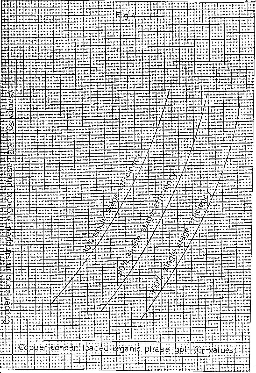
From the calculation method described so far it can be seen that the relationship between the stripped organic copper concentration and the loaded organic copper concentration can be readily calculated for different numbers of extraction stages and different values of single stage efficiency. A graph of the loaded organic copper concentration against that of the stripped organic for each condition of number of stages and single stage efficiency can now be plotted. A typical result showing a family of curves is illustrated in Figure 4
b. Interpretation of the Strip Equilibrium Isotherm
We have so far only considered the extraction system but, as the operation of the extraction system affects the operation of the stripping system and vice versa, consideration must also be given to the manner in which the two systems interact.
Like the extraction system, in which insufficient values are known to enable the system to be described precisely, the only constant values for the strip system are the strip equilibrium isotherm, the spent and advance electrolyte compositions and the range of loaded organic copper contents derived previously from consideration of the extraction section. The copper pick up of the electrolyte in the strip section is defined by the proposed operation of the tankhouse and as a consequence, the O/A ratio to be used in the strip section is a variable, unlike the situation with the extraction section.
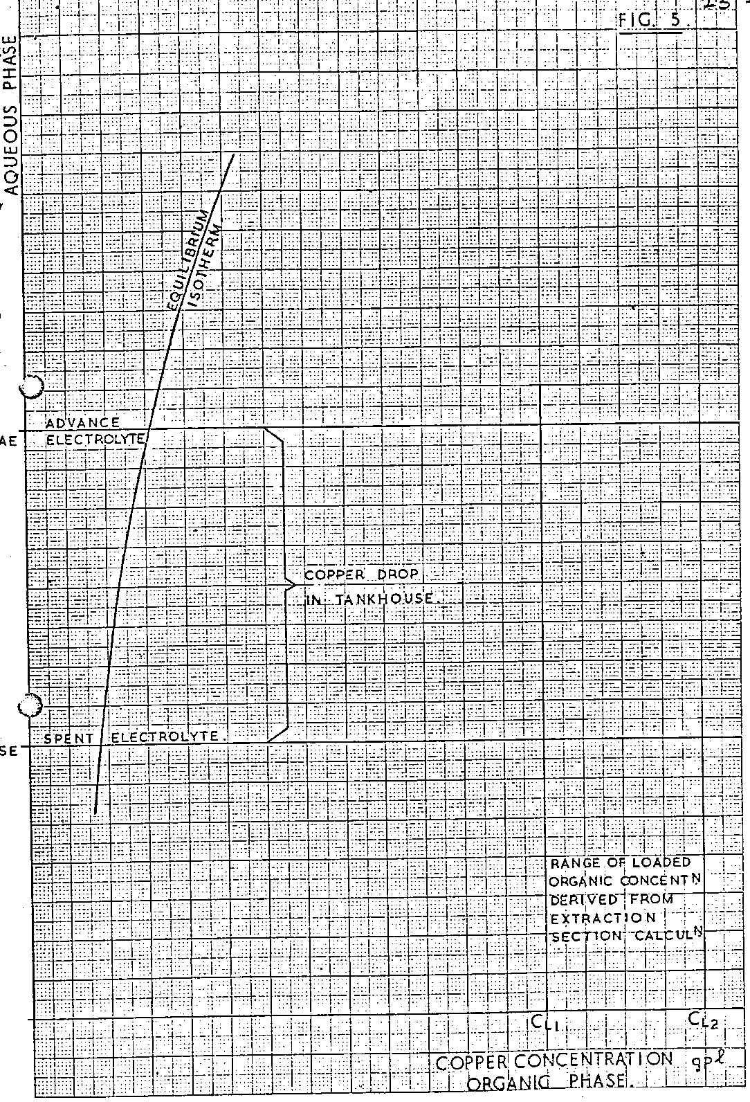
A typical LIX/copper strip equilibrium isotherm is illustrated in Figure 5.
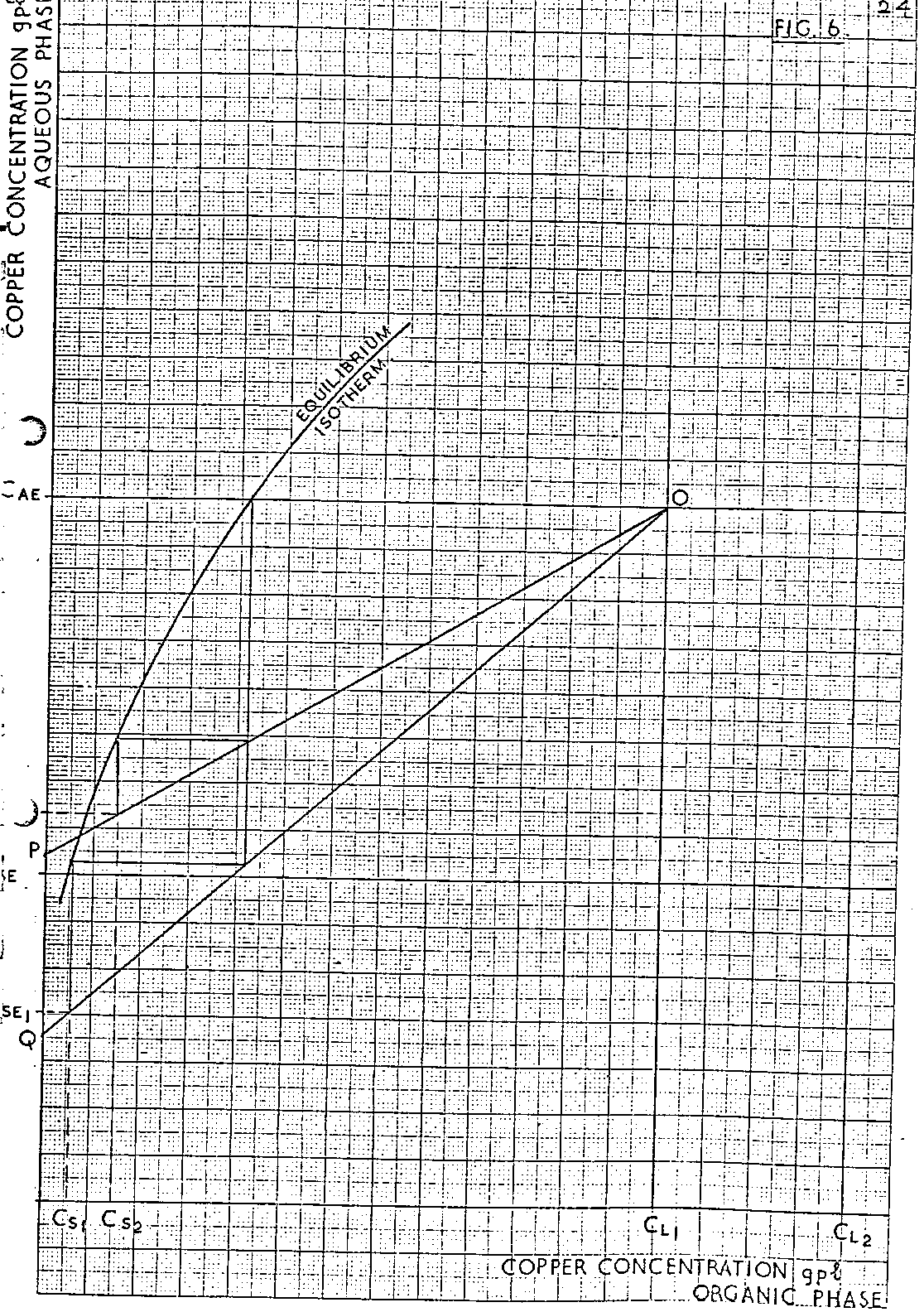
As with the extraction system, a relationship is drawn between the copper contents of the stripped and loaded organic solutions and, as there is a range of loaded organic copper contents to be considered, a range of related stripped organic copper contents should result. However, for the LlX/copper system operating with a two stage strip at 100% efficiency, the steepness of the strip equilibrium isotherm often results in the copper content of the stripped organic solution remaining constant, within calculation error, when the copper content of the loaded organic solution changes over the range of values derived previously from consideration of the extraction section. As stated previously, the precise slope of the operating lines in the strip section is unknown. The method of establishing the position of this line for ideal systems is described below and illustrated in Figure 6.
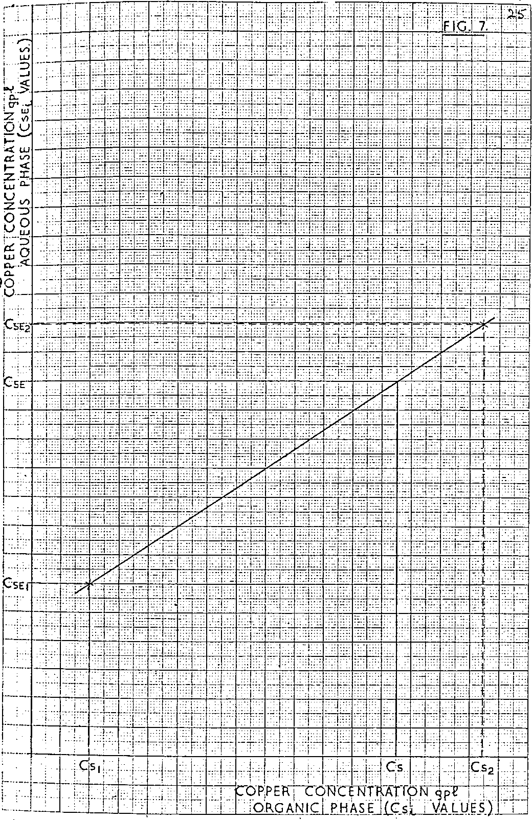
An operating line is drawn from point O to point P. The slope of the line, representing a particular O/A ratio, is chosen so that the required stage process (two in the diagram) results in the spent electrolyte solution inlet the system being of concentration C SE2, i.e. different from the required value for the spent electrolyte C SE. The corresponding stripped organic copper concentration C S2 is noted simultaneously. A second operating line OQ is drawn of such a slope that again for the required stage process, the spent electrolyte solution inlet the system is different from C SE. However in this case the line is chosen so that Q is on the opposite side of C SE on the ordinate to point P. The corresponding stripped organic copper concentration C S1 is read simultaneously. Plotting the related values of C SE1 and C S1 and inserting the required value of the spent electrolyte concentration, C SE, enables the corresponding copper content of the stripped organic solution to be determined, Figure 7. For most LIX/copper systems the relationship between C SE1 and C S1 will be a straight line. However if this is not so, further points may have to be derived by the method described above to enable the correct curve to be drawn as in Figure 7.
As for the extraction section, we have up until now only considered ideal systems, i.e. 100% efficient in all stages, but again real systems operate at lower efficiencies. To take account of this, a method identical with that used for the extraction section is followed and is described below.
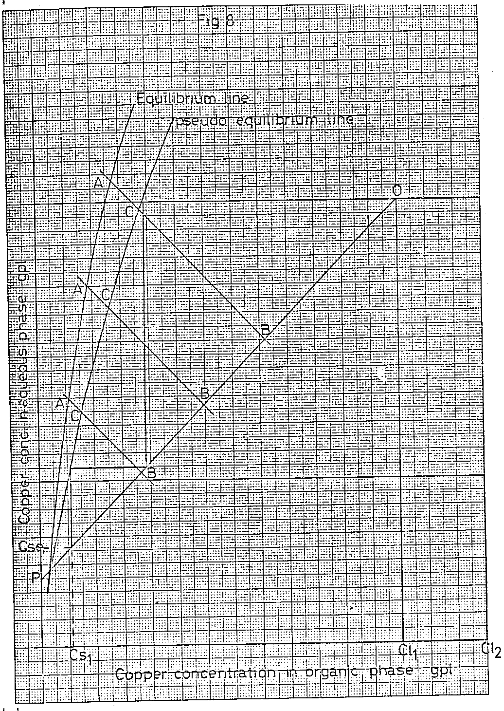
Draw, as illustrated in Figure 8, a series of lines intersecting the true equilibrium and operating lines whose slope is the reciprocal of the slope of the operating line. Measure the distance between the points A and B on these lines and multiply the values by the FACTOR calculated from the chosen single stage efficiency, as described previously for the extraction isotherm. Mark on the lines AB, point C the distance BC being the product of the distance AB and the FACTOR calculated as described previously. The pseudo equilibrium line can now be drawn through all the C points, including the intercept of the operating line with the true equilibrium line.
Having now constructed the pseudo equilibrium line, the values of C SE and C S can be determined as described previously.
The procedure is repeated for the other extreme loaded copper concentration CL2.
For many LIX/copper systems the steepness of the equilibrium isotherm results in no significant change in the copper content of the stripped organic over a range of loaded organic copper contents. This fact simplifies the calculation in that only two loaded organic copper contents need to be considered. However for systems where this is not the case, a minimum of three loaded organic copper
contents must be used to enable the accuracy of the method to be maintained.
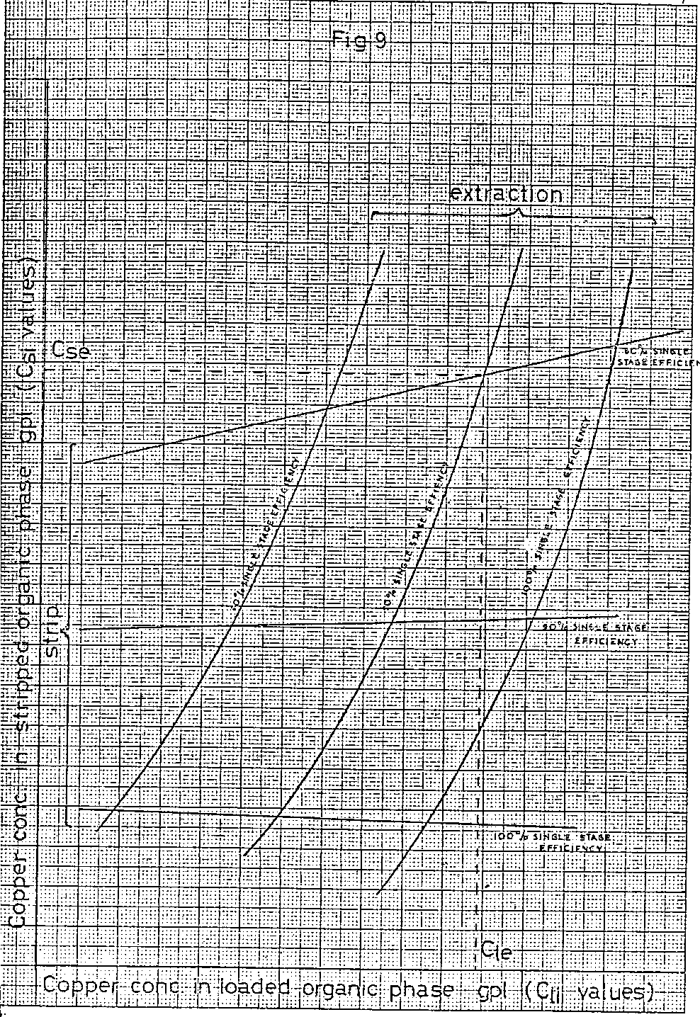
The resulting related values of copper in the loaded and stripped organic solutions are plotted on the same graph as the comparable figures from the extraction section calculation (Figure 4) to give a graph shown diagrammatically in Figure 9.
Each of the intersections on the graph in Figure 9 corresponds to the steady state copper concentrations of the stripped and loaded organic, solutions passing between the extraction and strip sections when each section is operating with the number of stages and the single stage percentage efficiency described. Thus the intersection detailed corresponds to an x stage extraction/y stage strip system operating at 80% single stage efficiency in the extraction section and 90% single stage efficiency in the strip section. The steady state concentration of copper in the stripped organic solution is C SE while that in the loaded organic solution is C Le.
These two values together with the extraction section O/A ratio and feed copper concentration can now be used to calculate the copper concentration of the raffinate, the efficiency of the whole system, the % extraction for the system described and the strip section O/A ratio in the following manner.
Subtracting the derived value of copper in the stripped organic solution from the derived value of copper in the loaded organic solution gives the amount of copper extracted into the organic phase.
C Le – C Se = C Ex
Multiplication of the amount of copper extracted into the organic phase by the O/A ratio in the extraction section gives the amount of copper extracted from the aqueous phase.
C Ex x O/A = C Ex A
Subtracting the amount of copper extracted from the aqueous phase from the concentration of copper in the aqueous feed gives the concentration of copper in the raffinate for the system as previously described.
C F – C Ex A = C R e
The % extraction can be readily calculated by dividing the amount of copper extracted from the aqueous phase by the amount of copper in the aqueous feed and multiplying by 100.
C Ex A x 100/C F = % extraction
The total system efficiency can be calculated using the following equation:
C F – C Re/C F – C Re* x 100 = Total System Efficiency
where,
C F = concentration of copper in the aqueous feed
C Re = concentration of copper in the raffinate under specified system conditions
and C Re* = concentration of copper in the raffinate under conditions of 100% efficiency in both the extraction and strip sections.
Finally the overall strip section O/A ratio can be calculated by dividing the copper drop in the tankhouse by the amount of copper stripped in the strip section.
Copper drop in tankhouse/C Ex o
Use of Equilibrium Isotherms using Overall Efficiency
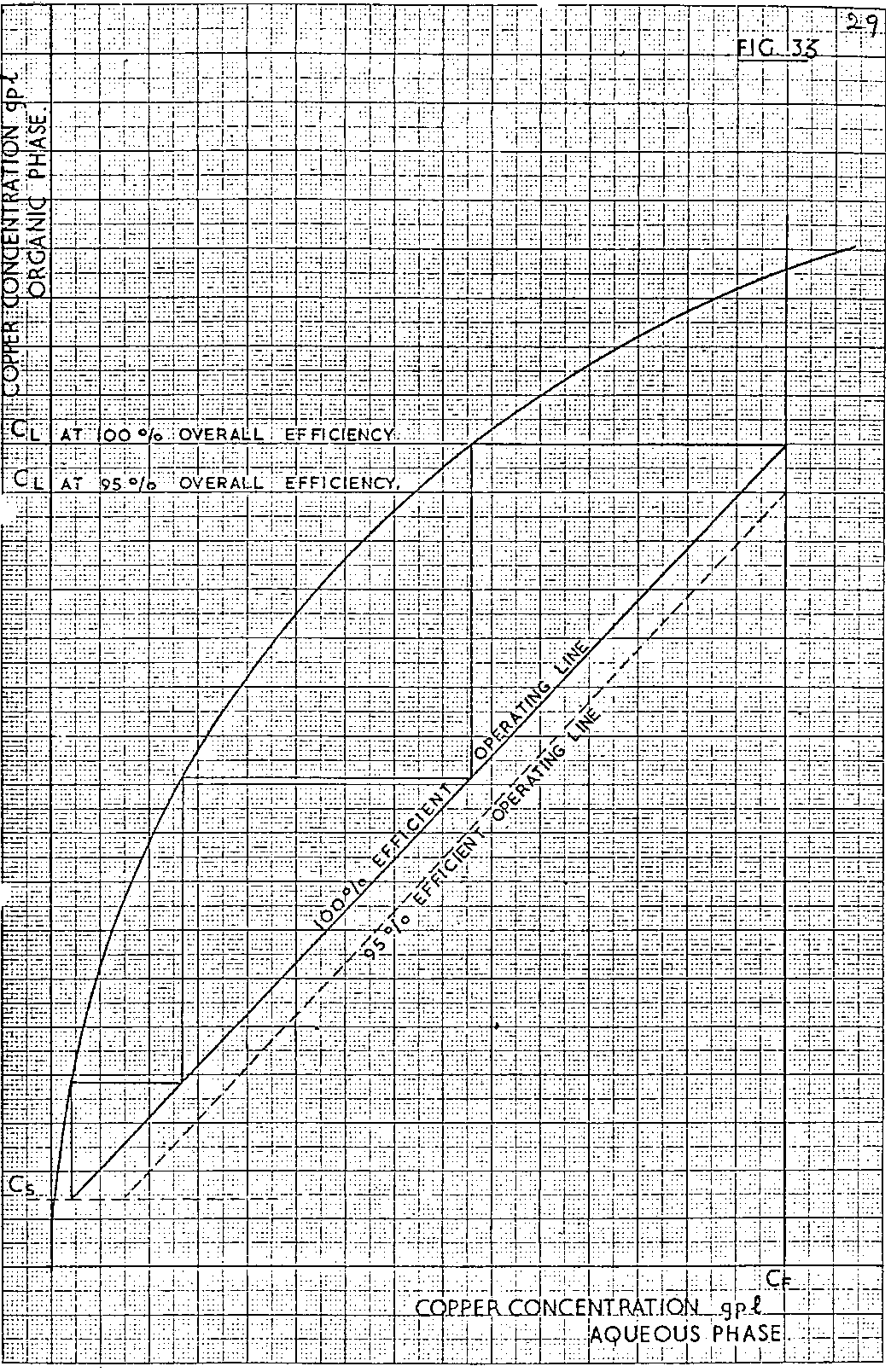
The construction is performed using the equilibrium isotherm and the operating line. This will give the number of stages and the compositions at 100% efficiency. The overall composition changes are C ORG and C AQ. Using an overall efficiency, these changes will be η x C ORG and η C AQ.
In Extract the pregnant liquor concentration will be known and a value for the stripped organic assumed and hence the loaded organic and raffinate concentrations are culculated. These points will lie, on a line parallel to the operating line. (see figure 33.)
Unlike the 100% efficient operating line the stepping-off procedure cannot be used for the 95% efficient line as a pseudo-equilibrium curve needs to be drawn. This is dependent on the individual stage efficiencies and it can be deduced from figure 33 that an infinite rariety of different individual stage efficiencies can be used to give the same overall efficiency.
Development of SX Design Parameters
For Proposals
The extraction and strip isotherms will be predicted from the CUAD curve. All others parameters will be estimated using the figures from previous relevant contracts as a basis.
For Contracts
The design parameters for a contract will be finalised by a programme of test work. This may include pilot plant results and/or laboratory testwork conducted by client or by DPG.