 The goal of the exploration program is to proof up resources and reserves and to estimate the value of what is being found. In short to answer the question; Can we make money from this pile of rocks or not?
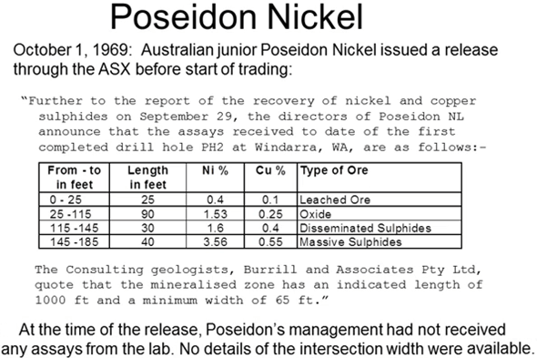
Some background to this question of resources and reserves. In 1969 the Vietnam War was in full swing and the demand for nickel was soaring. On October of that year, Australian junior Poseidon Nickel issued a release before the start of trading. Further to the report of recovery of nickel and copper and sulfides on September 29th the directors of Poseidon NL announced that the assays received to date are the first completed drill hole of pH 2 at Windarra Western Australia are as follows and they gave a table showing drill results with intersections broken down in ft. and nickel and copper assays to two decimal point. They continued the consulting geologists Burrill & Associates Pty. Limited quote that the mineralized zone as an indicated length of 1000 ft. and minimum width of 65 ft. It was later shown that at the time of the released Poseidon’s’ management had not received any assays from the lab, no details of the intersection width were available it was total fabrication.
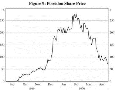
Poseidon management awarded themselves options before the announcement and Poseidon shares ballooned to almost 35,000% of their IPO value, management exercises sold the options before they revealed that the data was far too sketchy to draw any conclusions. When the actual assay results were released they were shown to be hugely overstated and with subsequent poor results the bubble dramatically burst.
It took ASA regulators nearly 20 years to do something about this problem but in 1989 they incorporated the first version of https://www.jorc.org/ JORC (Joint Ore Resources Committee) code, into ASA existing roles to standardize the method of reporting resources and reserves.
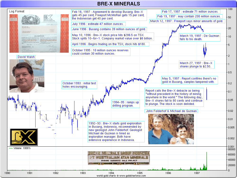
Then in 1997 the Bre-X scandal exploded onto the Toronto stock exchange for those not familiar with the story; Canadian David Walsh started a company called Bre-X minerals in 1989 but by 1993 he and his wife were declared bankrupt. That same year Bre-X minerals bought the rights to Busang Property in Kalimantan on the basis of a few anomalous grab samples. Walsh hired a Philippino geologist Michael DeGuzman to oversee exploration. Not much happened over the next two years but in 1995 reports of spectacular drill results began to be released. Over the following two years the resource estimates grew to 30,000,000 ounces of gold then to 40,000,000 ounces and then to 71,000,000 ounces. Share price climbed exponentially and the big mining companies were falling over themselves to get a piece of the action however they were having difficulty getting access to the project to carry out due diligence. In February 1997 there was a suspicious fire on site that destroyed most of the maps and assay sheets but that didn’t stop Bre-X from announcing that the resource could eventually reach 200 million ounces.
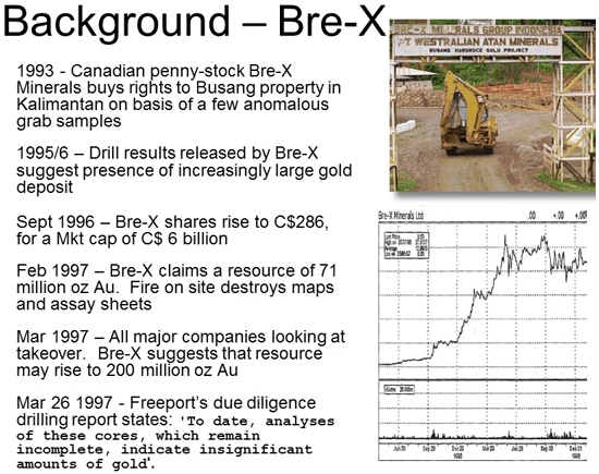
Shortly afterwards Freeport was finally able to get insight in re-assay core and Freeport reported soon after that to date analyses of these cores which remain uncompleted indicated insignificant amounts of gold. The Bre-X bubble burst and the share price tumbled. Michael DeGuzman was reported to have fallen from a helicopter although his body was never conclusively identified.
Now it was the TSX’s turn to be embarrassed and something had to be done. The following year the TSX set up a task force with a mandated to repair investors’ confidence by ensuring that there were adequate standards and disclosure procedures. That resulted in a seven-year discussion between the industry and players and regulators. In December 2005 national instrument 43-101 became effective.
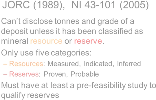
The Australian JORC and Canadian 43-101 regulations are very similar although the 43-101 is a bit more stringent on what must be disclosed. In basic terms both state that a company can’t disclose their tonnes and grade of a deposit unless it’s being classified either as a mineral resource or reserve. Resources become reserves as more data is required and confidence improves. Only five categories of resource and reserves are acceptable. For resources these are measured, indicated and inferred. For reserves they are proven and probable. Reserves must have at least a pre-feasibility to back them up and I’ll talk more about feasibility is later.
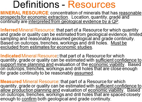
The mineral resources is a concentration of minerals that has a reasonable prospect for economic extraction; location, quantity, grade and continuity are interpreted from geological evidence by a QP.
Inferred mineral resources; one of those subcategories that’s part of a resource for which quantity and grade or quality can be estimated from a geological evidence, limited sampling and reasonably assumed geological and grade continuity. Based on outcrops, trenches, workings, and drill holes it must be excluded from estimates for economic studies.
The next one up from that is the indicated mineral resources which is that part of resource for which quantity, grade or quality can be estimated with sufficient confidence to support mine planning and evaluation of the economic viability, it’s based on outcrops, trenches, workings, and drill holes that are close enough for grade continuity to be reasonably assumed.
The top one in the resources is the measured category and it’s that part of resource for which quantity, grade or quality can be estimated with sufficient confidence to allow production planning and the evaluation of the economic viability it’s based on outcrops, trenches, workings, drill holes that are spaced close enough to confirm both the geologic and grade continuity.
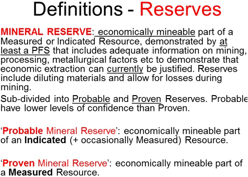
Moving now on to the reserves; mineral reserves are the economically mineable part of a measured ore, indicated resource and demonstrated by at least the PFS that includes adequate information on mining, processing, metallurgical factors etc. to demonstrate economic extraction can currently be justified and that word currently is very important. It has to be under current economic conditions. Reserves include diluting materials that allow for losses during mining and is subdivided into probably and proven reserves. The probable reserves are the economically mineable part of an indicated resource and sometimes in a measured one as well. A proven mineral reserve is economically mineable part of the measured resource.

Since a picture is worth 1000 words and this table summarizes resources and reserves. Projects rise up the Y axis as work improves geological knowledge and confidence and they move across the X axis with the addition of mining, metallurgical, economic, marketing, legal, environmental, social and governmental studies. Note the other areas in the middle of the center shows how they may change. Inferred resources cannot move directly to probable or proven reserves they have to increase to measured or indicated resources before they can be converted to reserves.
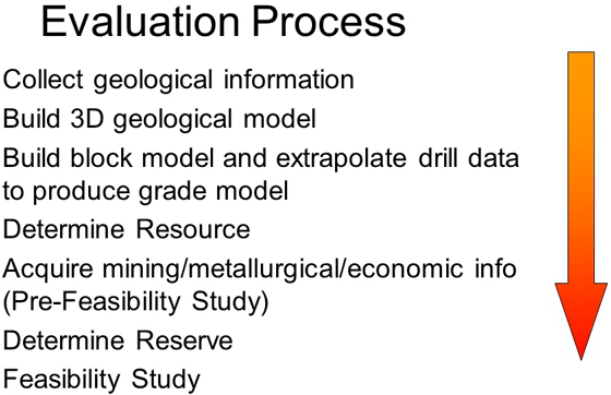
Raw exploration drill data into something useful, something that will eventually lead to the decision as to whether it makes economic sense to mine it or not. As you would imagine there are a number of steps that a project has to go through, this slide summarizes those steps and we will go through each one starting with the collection of geological information.

The first step is to collect all of the exploration data to select what can and what cannot be used in the next step which is the building of the geological model. Most of the data collected during the long process of exploration is used directly or indirectly into finding the geological model. Geological mapping, rock chip samples, trench data, geophysical data and drill log data may all have access to defining that geological model.
Soil sample although it’s rarely useful in identifying drill sites in the early parts of an exploration program is not actually much use into finding the geological model.
Once all the exploration data is compiled and the useful data sets are selected we can build that geological model. The geological model reflects the geologists understanding of the mineralization; its host rocks and its structural deformation. The geological model is built using 3-D modeling software the most important data comes from geological mapping and the drill database but other soft data can also be used and integrated this requires the model to use both a mix of data and geological intuition. His aim is to define three-dimensional envelopes that reflect characteristics that may impact on economics. For example the erosion surfaces, geological contacts or faults and one of the most important features he needs to model is the mineralization envelope. These features will all have direct influence on either the limits of the mineralization or on mining or processing costs; such as rock density, hardness or the degree of weathering.
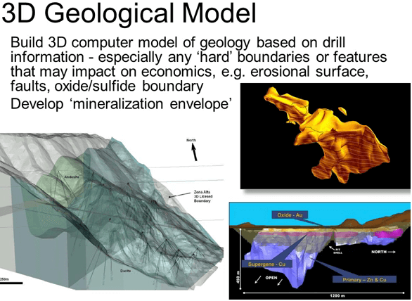
The mineralization envelope defines the outer limits of the mineralization it may have hard boundaries where the mineralization is known to be cutoff sharply by say a fault or soft boundaries which defined the outermost portions of the gradational fading out of the mineralization. In the case of soft boundaries the ultimate limits of mineralization will be defined later using just statistics to define where the grade drops below the applied cutoff.
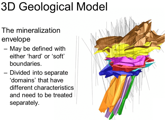
The mineralization envelope is sometimes divided into separate domains that have different characteristics and needed to be treated separately. There is no point in building and unnecessarily complex model showing every geological contact that may have been identified. If two rocked units have the same mining and milling characteristics they maybe clumped together to simplify the process.
Once the geological model is complete we move on to producing a grade model. Key to this process is the so-called qualified person or QP. The QP is defined as an approved engineer or geoscientist with at least five years of experience, who’s knowledgeable of the mineral property concerned and who has sufficient experience and qualifications to make the statements which are made within the report. He or she also has to be in good standing with the professional association and have recognized stature within that organization. The QP uses his professional judgment on a number of calls during the evaluation process and it is his professional and ethical reputation that’s on the line when he puts his name to a resource estimation.
The first step in constructing the grade model is to super impose a digital 3-D block model or framework onto the geological model, selecting block dimensions that allow sufficient detail. This is obviously a very course block model that I have in the illustration and it is just for illustration.
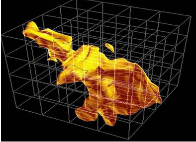
A real block model may have hundreds of thousands or even millions of rocks. The dimensions of the blocks depend largely on the size and the shape of the order envelope and it may vary within the model. Having established the framework we take the available assay data and extrapolate this to assign an estimated grade to every block in that grade model. Producing a grade model is a somewhat more restricted step than building the geological model. Not all the data that is collected during the long process of exploration and is useful in building that geological model can be used in defining the grade model. For resource estimation for example; chip samples assays cannot be used in a grade model, likewise not all drill samples such as those from air core can be used. Air core assays are not considered sufficiently representative for grade distribution due to their tendency to smear values.
Data from RC and Diamond drilling generally are acceptable even underground Channel sampling may be considered acceptable in certain cases. Before it is incorporated any data set needs to be carefully verified and any errors corrected.
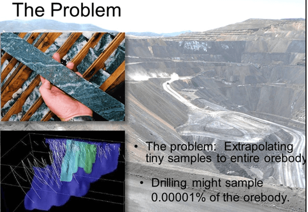
Now in grade estimation the process of extrapolating from the drill data to fill each of those blocks in the model has a fundamental problem that has to be overcome. A Diamond drilled core may have a diameter of say just 48 mm and yet we are trying to extrapolate that to full a block that may be tens of meters in each dimension and into the adjacent blocks as well. Drill core may comprise just 100th of a single percent of the ore body.

Selecting a representative sample is like having blind men trying to describe an elephant from the small portion that they can feel. Fortunately in the case of estimating grade we have a series of geo-statistical tools that can be used to assist.
What is estimation: It’s the process of using sample data to predict the most realistic distribution of grade or could be lithology or specific gravity or any other feature throughout the mineralized body. The only thing we know about our final grade model is that it will be wrong. We can never know the precise grade and distribution in any ore body until it’s been completely mined out and then it’s too late to be of use, however geo-statistical estimation can give us a reasonable idea of grade distribution in 3-D, hopefully good enough for us to base our financial calculations on it to allow a sensible go or no go decision.
There are a multitude of geo-statistical estimation methods:
- Polygonal
- Inverse Distance
- Kriging.
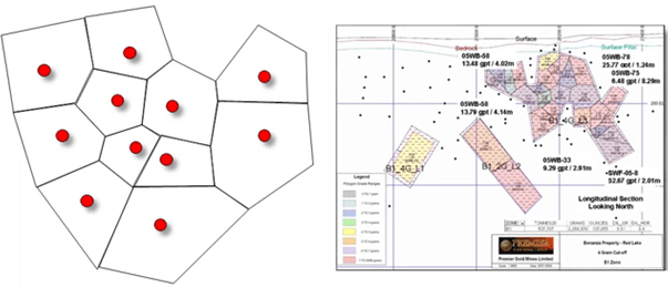
Polygonal methods: Polygonal estimations are very crude and rough and ready, there are several variants but basically they take known data points and then construct areas of influence around them assigning the grade of the sample point to the entire two or three-dimensional polygon. Here is a real-life example of a Polygonal estimate. Polygonal estimations are most commonly applied plain vein type deposits.
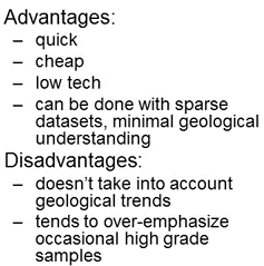
Another way to build up a polygonal method with the average grade of three samples at each corner of the triangles being applied to the polygon. The advantage of polygonal methods is that they’re quick, cheap and can be done with smart data sets and minimal geological understanding. The disadvantages are; that they don’t take into account geological trends and they tend to over emphasize the occasional high-grade samples. Polygonal methods are so crude that with easy access to 3-D software that incorporates relatively sophisticated geo-statistical code they are really seldom used now.
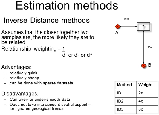
The next step up or the Inverse Distance or ID methods; this estimation method assumes that the closer together two samples are the more likely they are to be related. Using the straight Inverse Distant variant; if sample A is half the distance from the block to be estimated than sample B then sample A will have twice the weight of sample B. When assigning that grade to the block. In practice simple Inverse Distance still suffers from the same over emphasis of isolated high-grade samples that the polygonal methods suffer from. So ID squared or ID cubed is more commonly applied. These limit the spreading of their high grade. The advantages and disadvantages of ID methods are really very similar to those of the Polygonal methods although not as severe.
Kriging is by far and away the most commonly used methodology today. It’s named after a South African mining engineer Danie Krige who conceived the mathematical concepts in his Master’s theses. Like ID Kriging uses the weighted average of neighboring samples to estimate the unknown value at a given location but unlike the earlier methods it takes into account the directional trends that sampling exhibits, so that assays of samples in certain directions are weighted more heavily than those in other directions. Kriging is a two-stage process; the first this stage is to establish the predictable of sample values by comparing each sample with every other sample in the data set. To do this the computer plots each sample pair in a certain direction on a graph of distance apart on the X axis and against the variability of the pair on the Y axis. To produce a semivariogram then a best fit line is fitted through the points. The leveling off of the curve is the measure of the distance that a sample assay can be reliably extrapolated in that direction, in this case just 3.8 m. The process is repeated for other directions and the combination of these semivariograms defines a search ellipse showing how to weight samples in any particular direction.
The second stage of the Kriging process is to apply the search ellipse to estimate the grade of ensamples of blocks. This is done by taking the earlier define geological model with its super imposed empty block model and estimating grade within each cell of the block model using the ellipse to determine which assays are used in the process and how they will be weighted. Note that Kriging also provides a standard error to quantify confidence levels which may be important in classifying blocks is measured, indicated or inferred.
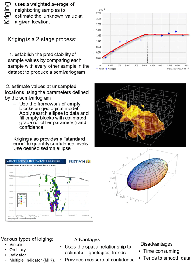
There are a number of variance in Kriging including simple, ordinary, indicator and multiple indicator the geo-statician will make a call as to which type of Kriging is one of the most best suited to the data set. In general the simplest variant that is suitable for a particular data set should be used. Multiple Indicator Kriging is one of the most arcane it was used by Snowden at Bruce Jack deposit and generated huge controversy but in this case MIK was justified by the unusually nuggety distribution of the gold in the Bruce Jack deposit. The advantage of Kriging is that it takes into account the real geological trends displayed by the samples and also that it provides a measure of confidence for each estimated block. The disadvantages are that it is time-consuming and tends to smooth the data somewhat. Individual blocks in the block model are not tagged with an estimated grade any number of characteristics can be attached to the blocks such as the rock type, rock density and hence tonnage, metallurgical characteristics, rock hardness which is of interest both to the mining engineers and metallurgist; metallurgical recovery and so on. Basically any factor that has a bearing on the cost of the mining or the cost of extraction of the metal should be including in that block model.

Now that we’ve built our block model that includes the grade we can use that to estimate a resource. Remember that the definition of a mineral resource is a concentration of minerals that has reasonable prospects for economic extraction. So first we need to work out what the likely economic cutoff is using an assumed metal price and the probable cost of mining and milling. Mining and milling any grade lower than this economic cutoff will result in an operating loss.
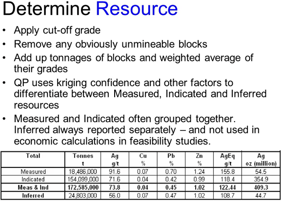
Only blocks with a grade of greater than the cutoff are used in the resource. The tonnage is, the remaining blocks are totaled and they are weighted and average grade is calculated to produce a total resource. Based on the Kriging confidence and other factors that the QP deems important this resource is divided into categories. Each of the blocks will have a measure of confidence assigned from the Kriging which is useful in determining where they classify them as measured, high confidence, indicated, lesser confidence or inferred – very low confidence. Measured and indicated are often clumped together in reports as they can be used in a pre-feasibility study. Inferred resources are considered too vague to be used in a PFS but they can be used in the less rigorous scoping study.
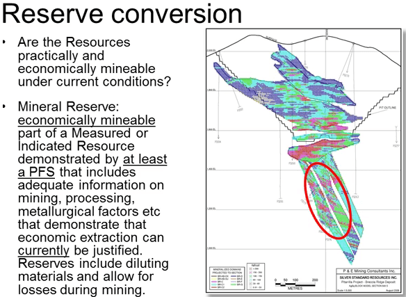
Although the definition of resources states that they should have reasonable prospects for economic extraction when they could be economically extracted is not defined. What we need to know is; are the resources practically and economically mineable under current economic conditions? Do they make the requirements to be classified as reserves? Very often the answer is no, for example this low-grade mineralization at depth is probably currently not economic.
To define reserves and produce a feasibility study we need more information than we currently have and we need to carry out additional studies to collect that necessary data. This data collection is normally done in three stages of increasing detail. The lowest level of detailed is the Preliminary Economic Assessment or PEA also sometimes called a Scoping study or Order of Magnitude study. This plugs in the first economic assumptions to see if the project makes any economic sense at all; inputs are rough usually within 40 or 50% and usually on the optimistic side so PEA although giving a useful first idea of the viability of a project should be taken with a pinch of salt.
Preliminary Feasibility Study or pre-fease or PFS as you will sometimes hear it called. This includes more detailed metallurgy data, including the processing method, associated capital, operating cost and percentage recovery. It includes rock mechanics; information to determine the pit slope stability and the angle of pit walls. In engineering data including the mining method, initial power and water requirements, their sources and capital and operating costs as well as softer social issues and costs. Cost estimates are generally plus or minus 20 to 30% for a PFS.
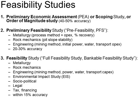
The third stage that will take us to the point where construction decision can be made is the Feasibility study sometimes also called a Full Feasibility study on a Bankable Feasibility study, they are all the same. This includes tightening up on all the above data to within 15% accuracy. It also includes an environmental impact study or EIS, sociopolitical studies, legal, tax and financing details. Once the PFS data has been collected the reserve estimate can be derived.
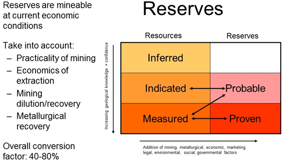
Reserves are mineable at current economic conditions. Portions of the resource are converted to reserves based on the practicality of mining, economics of extraction, mining dilution and recovery factors and metallurgical recovery. The resource statement may or may not include the converted reserves; check on this when you see both quoted to avoid double dipping. Generally Indicated Resources convert to Probable reserves and Measured resources convert to Proven reserves. The reverse is also true however and Probable reserves can be downgraded to Indicated or Measured resources if additional information warrants us at a later stage. As a general rule of thumb anything from 40 to 80% of a resource will eventually convert to reserves. If you see a figure that is outside of this range the resources were either highly over optimistic or seriously under drawed and both of these are warning signs.
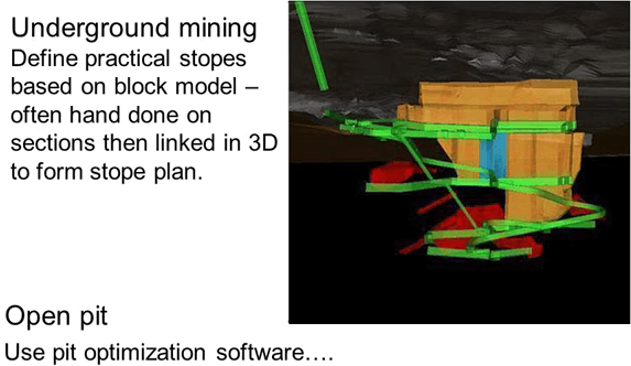
In the case of the deposit that will be mined from underground reserves are derived by defining practical underground stopes based on the grade block model. This is usually done by hand by a mining engineer using cross-sections. He outlines what can be practically mined based on the defined cutoff grade and physical mining constraints. These sections are then merged in 3-D to form the arc line of the plan stope. The blocks that fall within the plan stopes can then be total to form the basis for a reserve statement. In the case of a deposit that will be mined by open pit most of the process is done by computer nowadays, using mathematical algorithms to define the best pit shapes for multiple economics scenarios this process is called Pet Optimization.
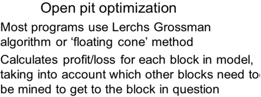
Most Pit Optimization software is based on the Lerchs Grossman algorithm or The Floating Cone method. This was most successfully applied by Jeff Whittle back in 1990 and you may hear engineers and geologists talking about a Whittle pit. The algorithm calculates the profit or loss for each block in the model taking into account which other blocks need to be mined to get to the block in question.
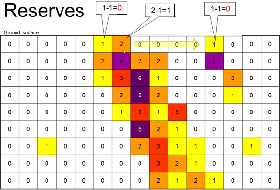
To illustrate this process let’s look at the simplified example using just a single vertical 2D slice through an imaginary block model. The numbers in the block show their in-situ value based on their grades and the selected metal price. I’ve color-coded them to represent this value. At the top of the model is the ground surface, now assume blocks cost 1 unit to mine and that our rock mechanics experts have said that rock will withstand 45° pit slopes. Starting on the top left and moving along the top line of blocks, no blocks have any value until we reach the first yellow block. This block has a value of 1 unit but it will cost 1 unit to mine and so it has a net profit of zero and it is not worth mining by itself. The orange block next to it however as a value of 2 units and it would cost 1 unit to mine so it would give a profit of 1 unit and so it would be selected for mining by the algorithm; I will mark it in bold. Continuing to move right along the top line no blocks of any value until we reached the last yellow block.
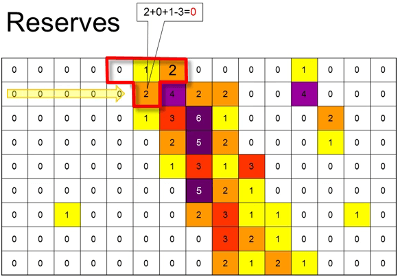
The computer then starts on the second row of blocks the first orange block has a value of 2 and to mine it would cost 1 however using 45° slopes the three blocks above it would also need to be mined adding the 1 unit credit from the yellow block directly above it which is not yet mined. The orange block above and to the right has already been mined and so is ignored in the calculation. That gives a total cost of the 3 units to mine it, with a total net value of 3, so the total profit of mining this block would be zero and the algorithm does not flag it for mining and passes along the row to the next the block.
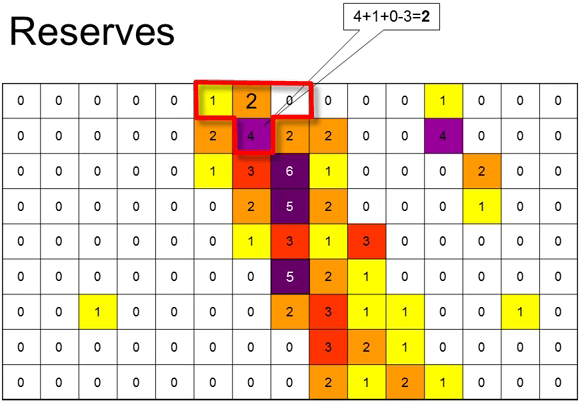
This purple block is a high-grade block worth 4 units again the three blocks above it need to be mined but the orange block is already being mined and is ignored.
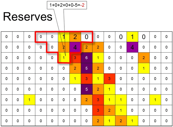
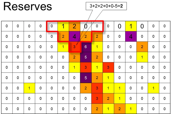
So the total net value of these blocks is 5 units, total cost to mine is 3 units giving a profit of 2 units. The block and those above it are therefore flagged to be mined. Flagging those blocks that are profitable to mine.
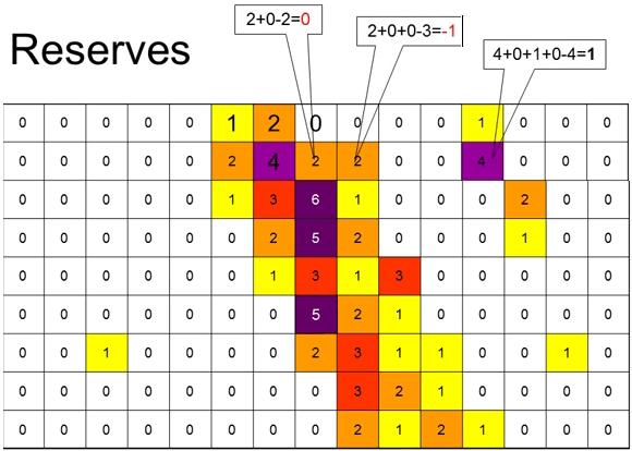
Until we come to the third row this time each block requires 8 blocks above it to be mined but some of these have already been mined or tagged for mining and are ignored.
Remember that although we are only showing this in 2D the algorithm is actually calculating in 3D so each of these triangles of blocks to be mined is really cone shaped.
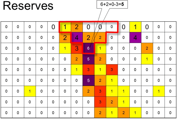
That is the floating cone that is sometimes applied to this process.

The process continues layer by layer steadily building up the shape of the optimal pit at the selected metal price and cost of mining.
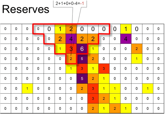
As you can see as we get to deeper blocks the number of blocks that need to be mined increases exponentially. Obviously this doesn’t matter too much in the center of the pit where many of the overlying rocks have already been tagged for mining.
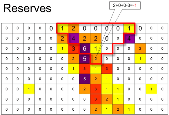
But it has a huge impact on the edges where blocks with minimum value are having to be removed to expose the worthwhile blocks and very soon the stripping ratio overwhelms the value of even the high-grade pods no more blocks can be mined.
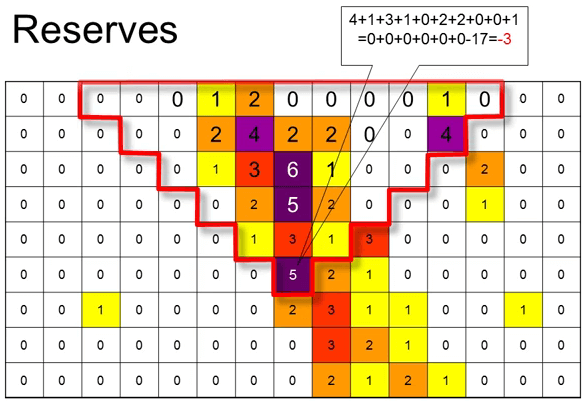
The final pit is outlined by the blocks that have been tagged from mining and mining this pit will provide the maximum operating profit. As I mentioned remember that this optimization is done in 3D a real block model may have well over 1 million blocks but the same principle applies.
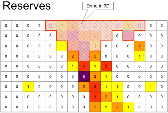
Once we have a pit to constrain the resource and current and realistic cost and prices have been applied we can convert some of those resources to reserves.
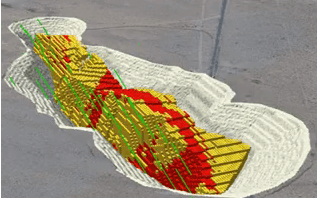
In fact the pit optimization process doesn’t produce just a single pit it produces multiple nested pits, each shell representing a different financial scenario.
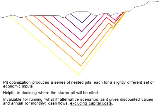
Because it is beneficial to start mining the most profitable pit first wherever possible these nested pits are incredibly useful as they show the most profitable pit shell – blue in this particular diagram; that can be mined as a starter pit and then a series of other pit shells that can be mined consecutively with push backs to the wall at each new phase. It also allows a series of what if scenarios to be run to see if their effects on the discounted cash flows, however remember that the inputs of a Whittle run are operating cost and product prices. Capital costs are not factored in and have to be applied separately. The most profitable Whittle pit shell may not be so profitable when the cost to capital included in the mix due to the stepped capex increases as through 38:14 is increased. Taking account of the capital costs takes place during the scoping and Pre-feasibility studies but it’s refined during the Feasibility study.

Now we come to the last step; the feasibility study. Armed with the reserves all the figures used in the PFS are then tightened up so that the cost is within plus or minus 15% accuracy. Assets that were only touched in the PFS such as the environmental and sociopolitical issues are dug into in great detail and the EIS or Environment Impact Study is compiled and submitted to the relevant authorities. All legal and tax implications are studied minutely. Financing possibilities are discussed with banks heads of agreements maybe drawn up or power and water supply and off take agreements may also be negotiated. The objective of the Feasibility study is to provide a tool that management and investors can examine and use to make a go or no go or an investment decision.
The reliability of Feasibility studies has been improved thanks to the NI 43-101 but even so the fact that the project has completed a positive feasibility study does not guarantee that it will be developed. There is plenty of positive feasibility on projects that are not economic and investors need to be very careful of taking published feasibility studies at face value. They need to dig into the details to see if the underlined assumptions that are being used are indeed realistic.
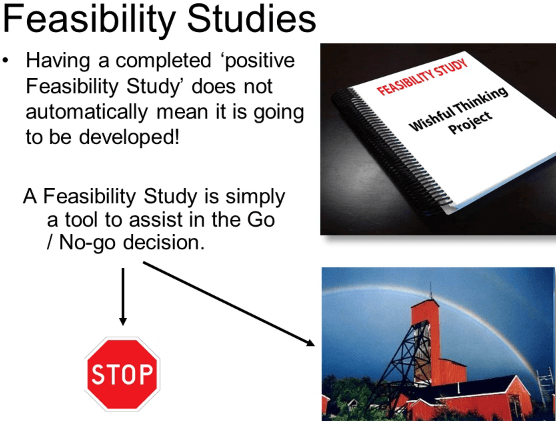
Mark Twain’s description of mining “A gold mine is a hole in the ground dug by a liar “ is a bit harsh but like most industries there are plenty of crooks out there. The 43-101 process is designed to make it harder for those crooks to operate but it’s not foolproof. A Feasibility study is simply a tool to assist in the go or no go decision. It’s a means to an end; it’s not an end in itself.
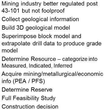
The mining industry is now better regulated thanks to the JORC and the 43-101 regulations that companies have to follow. The regulations make the evaluation of properties more transparent and standardized but they are certainly not fool proof. A project evaluation follows these steps; collect geological information including mapping, geophysics and drilling. Build a 3D computer geological model to display the extent of geological units that are significant for mining or processing. Superimpose an empty block model and extrapolated the drill data to produce a grade model using this geo-statistical method such as Inverse Distance or Kriging. Determine the resource dividing into measured, indicated and inferred categories according to confidence levels. Acquire mining, metallurgical, economic information to be able to make the basic economic assumptions.
A PEA has an accuracy of plus or minus 40 to 50% a PFS has an accuracy of plus or minus 20 to 30%. Also remember that the PFS can only use measured and indicated resources. Determine the reserve by designing stopes or optimizing a pit and including only those resources that fall within the mining plan. Use those reserves and improve cost and data to within 15% now as the basis to produce a feasibility study and finally we come to the construction decision remembering that a positive feasibility study does not necessarily mean a positive construction decision.
