In the operation of today’s large scale ore-processing mills, it is extremely important to have some way of making an objective evaluation of the performance of the available flotation reagents. While Reagent Testing the use of Statistics is necessary for Result Analysis. Attempts to do this may often result in inconclusive findings since the magnitude of the difference in the mill results for any two reagents is apt to be quite small compared to the variability introduced by the process and the analytical procedures used to measure them. In cases where two reagents give vastly different mill results, evaluation becomes a simple matter and as such deserves no further attention here. A question of primary concern, however, is how a mill can go about evaluating the performance of two reagents which may, for example, give a difference of only 0.0017, copper in the tailings or of 0.2% in copper recovery. The casual observer may feel that such small differences may be of little importance, but in a mill whose daily tonnage is between 30 and 40 thousand, these differences could mean a substantial savings.
Any comparison which is made regarding the metallurgical performance of two reagents will be made on the basis of assays performed on samples of the heads, tailings, or concentrates taken on-stream in the mill. The results of these assays will fluctuate about some average value from day to day reflecting not only the analytical uncertainty, which may be quite small, but also small variations in ore composition, reagent dosages, temperature, feed rate, and pH.
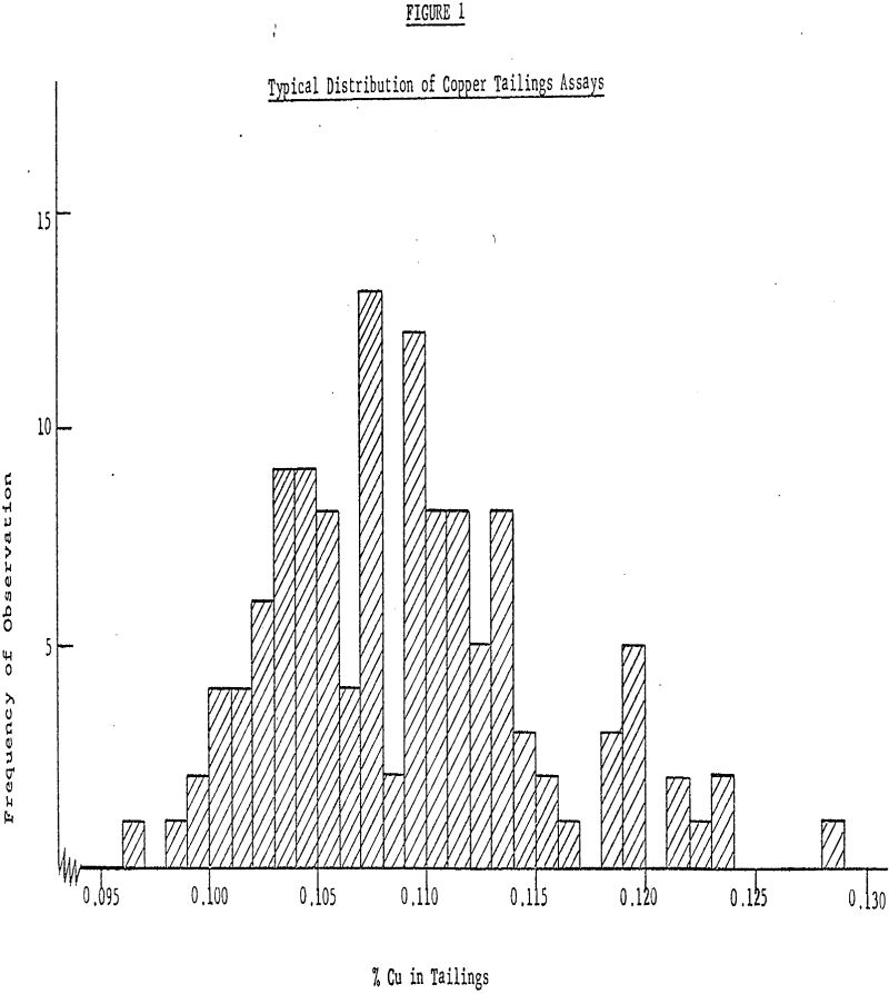
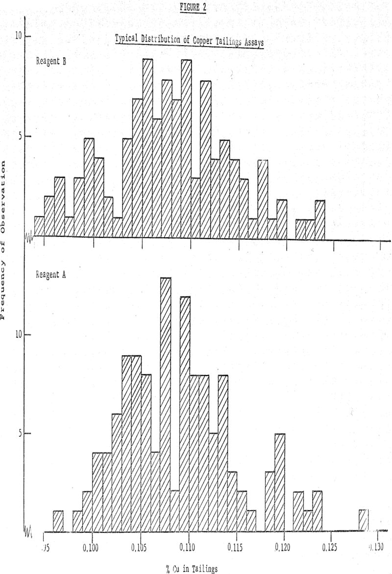
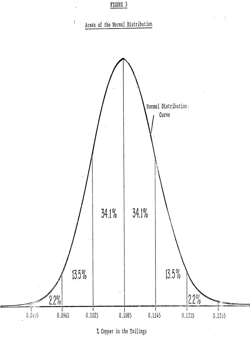
The average tailings assay of distribution A is 0.1085% with an estimated standard deviation of 0.0060%. The standard deviation indicates how widely scattered the observations in the sample were and gives an idea of how widely scattered future measurements are likely to be. If the usual assumption is made that the observations have deviations which are well approximated by the so-called normal distribution, then from an estimate of the standard deviation based on this, large an amount of data we can expect, roughly 68% of past and future values to fall within one standard deviation (±0.0060) of the mean roughly 95% to fall within two standard deviations (±0.0120) of the mean and roughly 99% to fall within three standard deviations (±0.0180) of the mean.
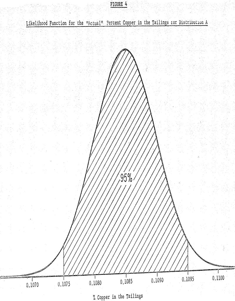
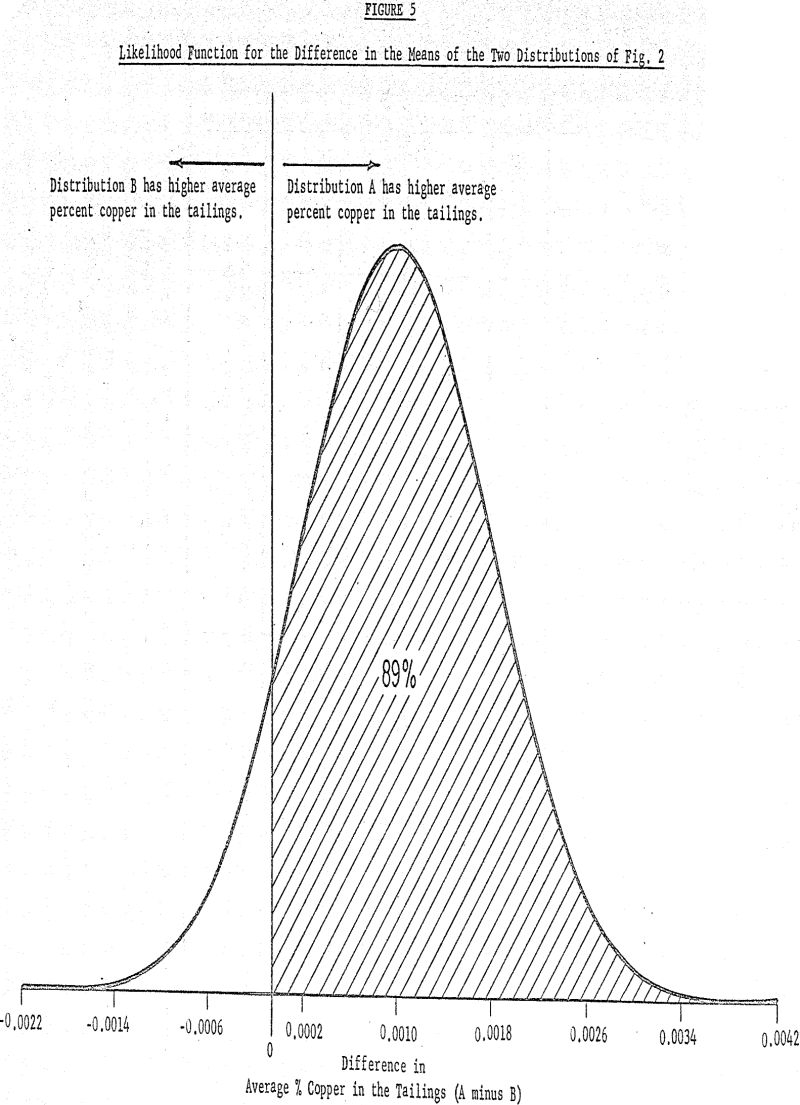
The arithmetic average of the distribution is 0.1075% Cu with a standard deviation of 0.0064% and as previously given, the average of the lower distribution (reagent A) is 0.1085% with standard deviation 0.0060%. If the only question is whether the two distributions are different, the likelihood function shows that there is a 0.89 likelihood (i.e., 89% chance) that the difference in the averages is positive (i.e., distribution A has a higher average than distribution B).
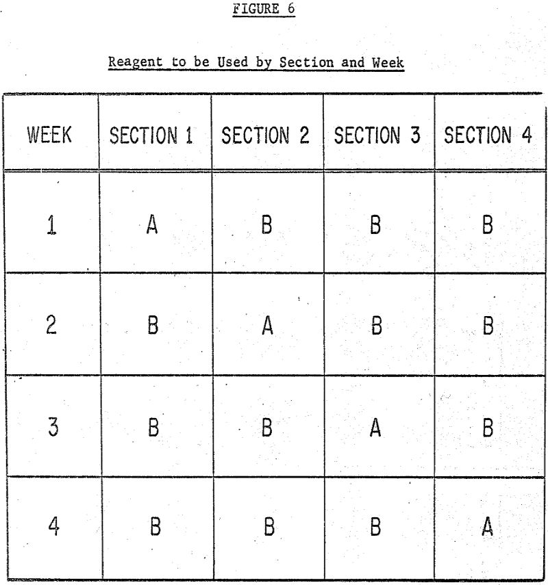
As an example of how these simple statistical tools may be used to evaluate small differences in reagents, details will be given of a test which took place at a large southwestern copper mill in June, 1962. The mill was interested in evaluating two reagents (denoted here as reagent A and reagent B) to determine which, if either, gave superior metallurgical results. From observation of the results, of previous tests, reagent B seemed to be the superior one. These previous tests, however, were not run in such a way as to permit a direct comparison to be made that is, each reagent was used in the entire mill for a period of time and the results compared with-data from a test in which the other reagent was also used in the entire mill at some other time. Further more, since the data were not subjected to a statistical analysis, objective statements could not be made concerning the difference in performance, i.e., the certainty with which this”difference could be established.
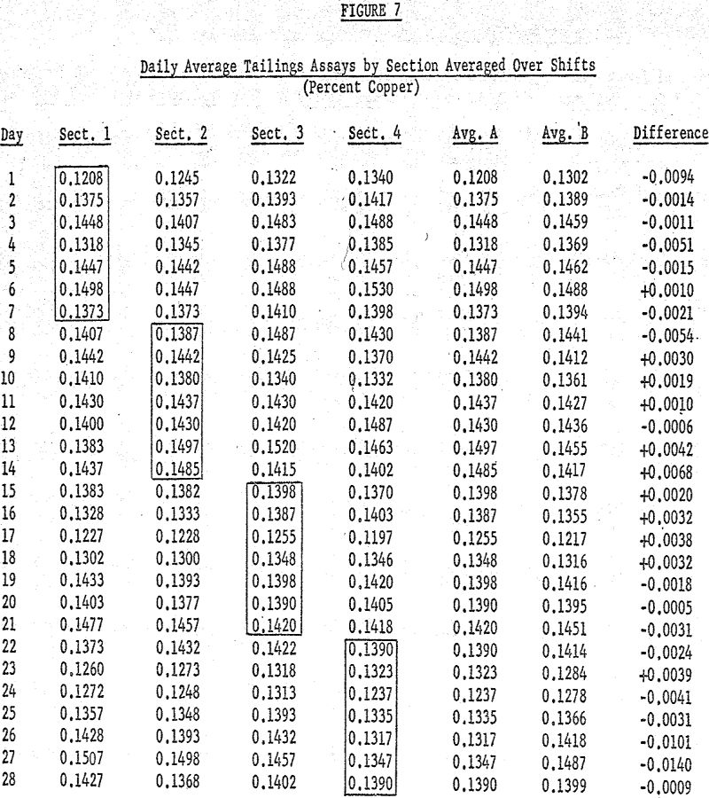
On June 1 the average % copper in the tailings sample when reagent A was used was 0.1208% (the average of the tailings assays for the three shifts of Section I). For the same day the average tailings assay for samples of ore floated with reagent B was 0.1302%. This procedure was followed for each day of the four week test for the following properties:
- % copper in the tailings
- % copper in the heads
- % copper in the concentrates
- % recovery
- %+65 mesh in the flotation feed.
Question one is easily answered by the arithmetic average of the differences. The results show that on the average reagent A gave
- lower % copper in the tailings by 0.001%
- lower % copper in the concentrates by 0,11%
- higher % recovery by 0.20%
- finer grind, i.e., lower % + 65 mesh by 0.09%
while floating ore with heads which contained an estimated 0.001% more copper.
The likelihood functions for head and concentrate assays and for grind (% + 65 mesh) tell a different story than those just seen. Whereas in the previous cases the likelihood was high that the difference was either positive or negative, in the likelihood function for head assays there is only a 0.62 likelihood that the difference is positive (i.e., reagent A was used on ore with higher head assays than the ore floated by reagent B). This, of course, means that there is a 0.38 likelihood that the opposite is true, and lends strong support to the hypothesis of no difference.
On the other hand, however, these same people will quickly draw conclusions if they realize that there is only a 5 to 10% risk of being incorrect, particularly if actions based on these conclusions, if correct, may result in substantial savings.
Thus, armed with the knowledge provided him by the likelihood functions the mill manager is fully aware of what he may expect to gain from one reagent as opposed to the other. From this point on, the decision of which reagent will be used depends on a weighing of expected gains against such things as differences in cost and other properties of the reagents not directly associated with their metallurgical performance.
A more subtle answer involves a change in the design itself. As indicated earlier, the optimal design for a mill with four parallel flotation circuits would call for using reagent A on two circuits and reagent B on the remaining two. This change alone would reduce the spread of the likelihood function by 13% of what it was in the “one circuit for A, 3 circuits for B” setup. Combinations of the improved design with increased testing time would, of course, give even greater reductions in the uncertainty of the conclusions.
Answers to question two are as numerous as are the mills for which the test would be designed. Therefore, only an outline will be given here of what might be done in mills with fewer flotation circuits. Several plans including the one discussed are given in the Appendix together with the appropriate analysis methods.
The one-circuit mill quite obviously cannot test both reagents simultaneously. However, this does not mean that a reagent testing plan cannot be designed for such a mill. It will be recalled that the primary objective in designing a test was to give each reagent the opportunity to float as nearly the same ore as possible at as nearly the same time as possible. If this same idea is followed for the one-circuit mill. This outline should be followed for the first four days and then repeated as many times as necessary to establish the desired difference in reagents.
