One of the Bureau of Mines missions is to research the techniques required to achieve structural and environmental control of all mill tailings disposal, both surface and underground. Correlatively, then, the Bureau attempts through advanced practices to reduce jeopardy to life and property. The investigation reported herein stressed the surface-control aspect of this research, whereas other Bureau projects have concentrated on underground disposal.

As a consequence of several developments in the mining industry in the last 10 years, tailings disposal, hitherto practiced with scant attention to environmental problems, has become as important in mining operations as drilling, blasting, milling, and haulage. Frequently, an otherwise valuable ore body is not considered minable unless adequate disposal of mill wastes can be accomplished. New and increasingly stringent restrictions have been precipitated by public alarm and the consequent demand for complete environmental quality control. To support these demands, new environmental and pollution control laws are being passed by Congress, moving more speedily now and encouraged by a Presidential request for billions of dollars to purify the earth, air, and water for the maintenance of ecological balance.

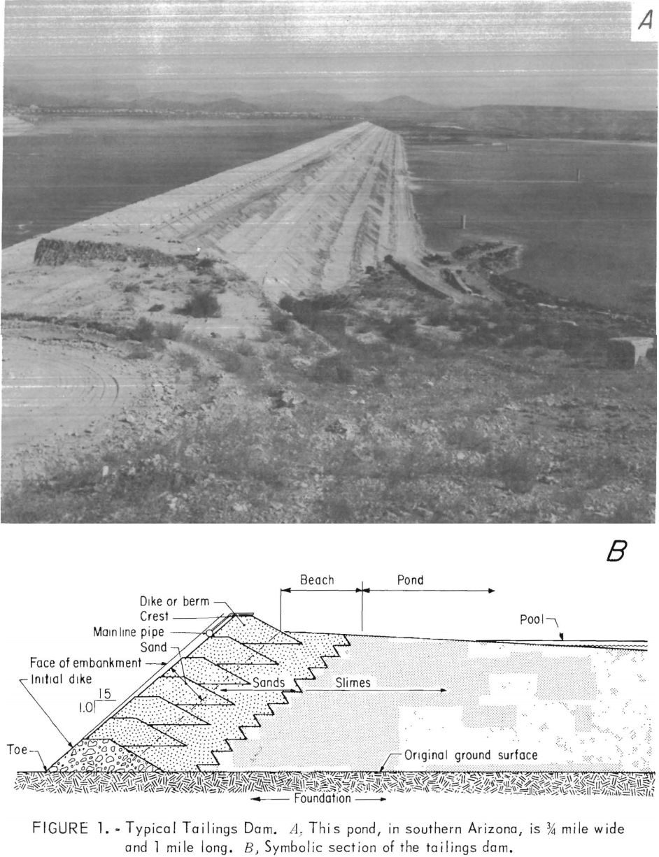
A second factor which has made tailings disposal so critical today is the utilization of large mining equipment as opposed to the smaller equipment used in the past. Huge open pits are now operating at a steadily increasing rate; these create great volumes of waste and mill tailings, which must be systematically disposed of. Because the disposal piles are massive, they can be very hazardous. Figure 1A portrays the extent of a typical tailings pond. Part B of figure 1 is a symbolic section of a representative pond.

The occurrence of failures throughout this country and South America and the widely published disaster in Aberfan, Wales, has brought mill-tailings disposal to the forefront of attention. The Aberfan disaster occurred when the waste pile failed and destroyed a small schoolhouse, killing most of the children inside. Preconstruction engineering studies of such embankments are essential for maximum safety. As mining progresses and waste dumps grow higher and larger, the probability of failure steadily increases, for slope stability and the factor of safety concomitantly decrease.

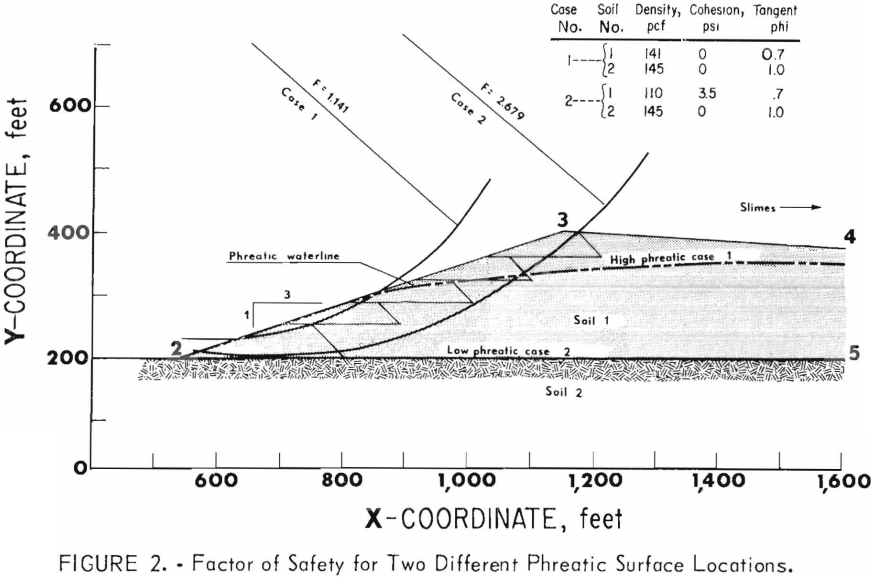
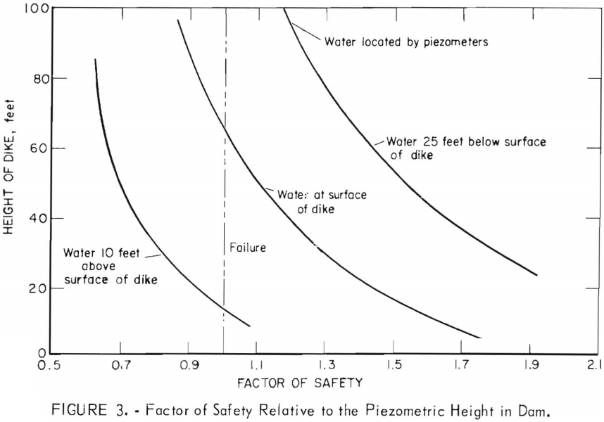
Closely related to the factor of safety of these embankments is the location of the phreatic water surface. The relation of the height of the phreatic surface to the factor of safety can be determined by the Bishop method of slope-stability analysis. Figure 2 portrays the tremendous difference in the factor of safety (F) for a low phreatic surface (at ground elevation) versus a high phreatic surface. The factor of safety drops from a safe 2.6 to a dangerous 1.1 as the phreatic surface rises to the elevation indicated. Figure 3 illustrates the relationship between the factor of safety and the height of a dike and the height of the piezometric water surface relative to the embankment surface. A review of the history of failures throughout this country reveals that in most cases water was the incipient factor that propagated the failure of these embankments. Consequently, the need arises for a reliable method of predicting the location of the phreatic surface within a mill-tailings embankment. Further, for environmental pollution control, a method for predicting the rate of water movement in and about a tailings pond would be highly desirable.

Finite-element, mathematical models that solve LaPlace’s and Richard’s equations numerically were used to locate the phreatic surface within tailings pond embankments and to define the subsurface flow of water from the pond.

Both must be known to design structurally and environmentally safe tailings dams. The permeability distribution within and beneath the embankment, the fluid potential values upgradient and downgradient from the embankment, and the geometry and elevation of an approximately impermeable layer at some depth beneath the embankment were used as computer inputs in analyzing over a dozen finite-element models of tailings dams varying structurally from simple to complex.

Results predicted with the finite-element model were confirmed with measurements in a laboratory model of a tailings pond and in the field. Of particular importance to the design of safe slopes, all data indicated that the phreatic surface within a tailings dam is concave upward, a configuration opposite that in most earth dams. The close correlation between predicted and experimental values confirmed the practicability of using the finite-element technique to design safe tailings dams.

This investigation proposed to utilize recently developed, mathematical modeling techniques to provide the solution to the problem. It should be

emphasized that the primary purposed was to develop and illustrate the application of the technique, not the basic soil parameters required for total solution. To the best of our knowledge, the technique described herein has never been applied to mill-tailings dams. It is based upon a finite-element method of numerical analysis, which is employed to develop mathematical models of mill-tailings disposal dams. The testing and data gathering were carried out for 2 years in order to develop enough parameters to build a realistic model. This study, in itself a complete research project, will be continued by the Bureau of Mines to further define these various parameters for various types of ponds. The finite-element procedure described in this paper can also be applied to many other mining problems, such as the dewatering of pit walls and water control in underground fills and in underground mining operations.

Review of Tailings Pond Design

A complete description of standard tailings disposal practices is documented in Kealy and Soderberg. The study is based upon personal inspection of all major mining districts throughout the United States and Canada; the report describes current problems and remedial techniques. This study convinced the present writers of the need for a seepage-prediction analysis.

Very little literature has been published on tailings disposal systems. Most of the publications are in mining magazines, although a few unpublished consulting reports are available. All of the available articles are discussed in reference, noted before. During the literature search it became apparent that most engineers currently designing tailings disposal systems are with consulting firms that traditionally design water-retaining dams; consequently they apply many of the same techniques and the same assumptions used in ordinary dam construction.

After considerable exploration it became apparent that many of these assumptions are not appropriate. Tailings, produced by mill crushing, screening, and sizing, have different characteristics from earth. Further, because of the type of construction used in tailings ponds, the flow lines and potential boundaries must be treated differently from those in a standard dam.

Figure 4 shows that an equipotential line in a typical dam construction becomes a flow line in a mill-tailings disposal unit. In addition, the standard Dupuit parabolic configuration for the phreatic surface normally does not occur in a mill-tailings dam. The location of the true phreatic surfaces

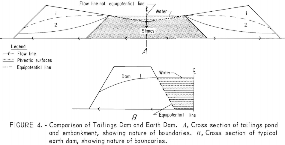
customarily lies closer to line 2 than to line 1, This placement has been misinterpreted throughout the industry. Evidence for these statements will be documented in the text of this report.

It is apparent from literature research and field investigation that industry has conducted, or sponsored, few soil mechanics studies on tailings disposal systems. Rather, companies have relied heavily upon consultants traditionally working in dam construction. In the past (and somewhat presently), operating firms have been solely concerned with getting the ore out and simply getting rid of the tailings as quickly and easily as possible-a standard policy in most small operations.

Methods of determining slope stability were also researched for this investigation. Much work in this area has been done in universities and a few consulting agencies. Excellent techniques for predicting a factor of safety are now available, and these procedures are being used in the construction of new tailings disposal units. However, in many of the cases reported, little concern was given to water location and its profound effect upon stability.

The authors found no technical literature that considered pollution by water seepage through mill-tailings dams.

The traditional method of describing a flow system in a dam is the flow net sketching construction method, which was developed much earlier by soil mechanics engineers and hydrologists. This technique, however, can be applied only to homogeneous, isotropic materials, except for a few simple cases in which it can be used for anisotropic conditions by a change of scale parameters. For tailings disposal dams that are truly anisotropic, the flow net sketching method becomes very cumbersome, if not impossible, to use.

Hydrogeologists and hydrologists have also utilized various types of resistance boards (analogs), both two and three dimensional, as tools for describing water movement in substrata. These analog techniques have also served for interpreting water movement in and beneath standard water-retaining dams. Based on analog experiments conducted at the University of Idaho and on the literature, it was found that these devices become quite cumbersome since one must deal with physical equipment. Therefore, great control is not readily obtainable. They do, nevertheless, have a great advantage in that one can readily detect gross errors; thus they will remain as a check or initial step in a more complicated finite-element, computerized analysis.

Toth, utilizing a theoretical analysis, describes regional and interregional waterflow systems based upon individual watersheds. His work occasioned further work by Freeze and Witherspoon, who used a finite- difference technique that handled anisotropic conditions. It is strictly an analysis of basin flow systems and thus has different boundary conditions than does the mill-tailings problem researched here. Their analysis of the effect on flow of various heterogeneous, anisotropic, porous media within a region is of great interest and was certainly beneficial to this study.

In any of these techniques-flow net sketching, analogs, analytical techniques, and finite-difference techniques-only a limited number of parameters are required for solving the flow problem. These are (1) permeability (if the body being studied is anisotropic, permeabilities in both horizontal and vertical directions) and (2) the boundaries of the body in question in terms of hydraulic heads and locations. The testing techniques for obtaining permeability values both in the field and in the laboratory are well documented.

More recently, new techniques for determining anisotropic permeability in the field by analytical mathematical methods have been developed by Weeks and Dagan. For the studies contained herein, however, these methods were not utilized because they simply cannot handle complex permeability distributions. The data for this paper were obtained using standard soil mechanics techniques and other Bureau research. A rough approximation of the correlation of the data was made so that the model could be developed.
(The specific methods and areas tested will be described later in the text.)

Summary of the Finite-Element Theory

The finite-element technique is a numerical method of analysis whereby the region of interest is divided into discrete elements. Originally the method was applied to stress analysis. Subsequently, the system was heavily used in structural engineering for stress analysis. A discrete solution, versus an analytical (or continuous) solution, provides answers to a problem only at discrete points in the body under study rather than a continuous solution, which is obtained by the analytical method. In most instances, discrete solutions are adequate, and they permit the treatment of complex boundary conditions. Further, they allow one to obtain approximate solutions to problems that cannot be obtained via analytical approaches. Zienkiewicz provides fuller discussion of the intricacies of this methodology.

The first publication treating the application of the finite-element technique to seepage problems appeared in 1965. This article presents the basic theory upon which future seepage studies and computer programs were written. Concerning the accuracy of this practice that is, the accepted accuracy numerous waterflow problems have been compared analytically and numerically by the finite-element method. The two methods show excellent agreement. It should be stated, however, that in all of the published studies all the boundary conditions were known. No free water surfaces were determined in these analyses.

Finite-Element Models with Free Water Surface

In this study the basic finite-element theory was adapted to the selection of the free water surface. In 1967, at approximately the same time, both Taylor and Brown of the University of California at Berkeley and Finn of the University of Vancouver utilized a matrix to develop a free-surface formulation by employing the finite-element method. Finn made use of the finite-element technique, coupled with the trial-and-error method of locating the exit point of the phreatic surface-accomplished by relocating the exit point after each trial. Taylor also developed a technique for finding the phreatic surface; however, his work was done without the trial-and-error location of the exit point. After studying the various approaches to the problem, the present researchers decided that Taylor’s technique is the most versatile and logical.

Theory of Darcian Flow

This section is directed to developing the mathematical theory and associated numerical analysis (finite-element procedure) for the seepage problem outlined earlier. The objective is to provide potential users with insight into the formulation of the computer program utilized.

Isolation of Region of Study

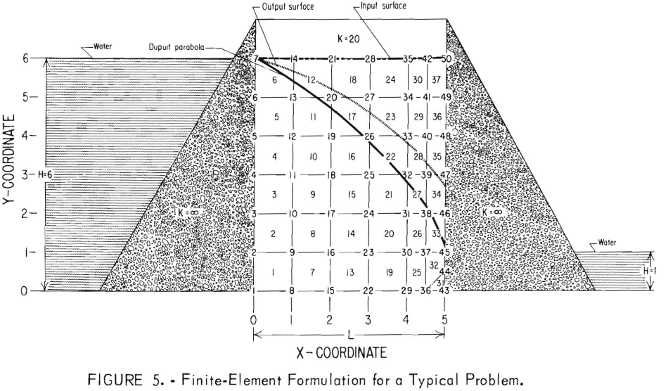
The first step in the analysis is to define, or isolate, the region of study in terms of boundary conditions. The effects of these conditions on flow and the relationship of the various elements can then be determined as illustrated in figure 5, where 37 finite elements are delineated by 50 nodal points. Boundaries are specified by the geometry of the problem: (1) an impermeable base (nodes 1, 8, 43); (2) a hydrostatic upstream equipotential line (nodes 1 through 7); (3) an estimated initial free surface (nodes 7, 14, 21, 50); and (4) a downstream equipotential line (nodes 43, 44, and 45).

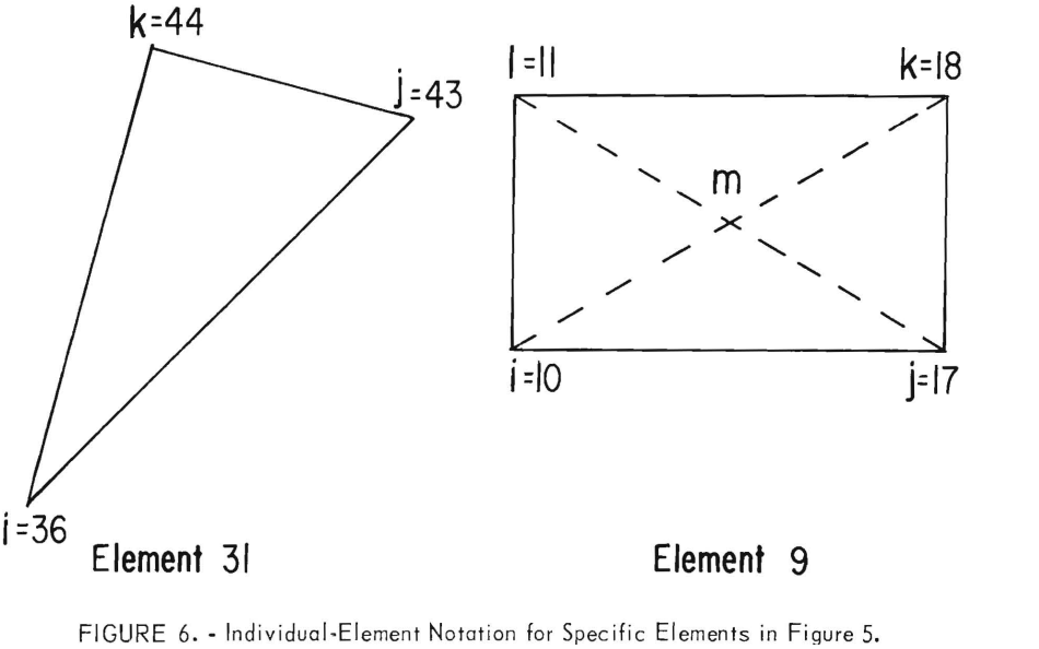
For the approximate solution to this problem, the flow region is divided into 37 elements. An element consists of a plane triangle with nodes at each vertex. Quadrilateral elements can also be used since this figure can be sub-divided into triangles to conform with elemental theory. The program subdivides the elements automatically. Note that in figure 6 node M is automatically placed within the quadrilateral via programing; this placement simplifies element net construction.

 

Darcy’s Law in Terms of Pressure and Gravitational Potential

The theory of waterflow through porous media is based on the classical experiment originally performed by Darcy in 1856. Mathematical models may be validly used only if Darcy’s assumptions hold true.

Darcy’s law is expressed as follows :

q = -ki,……………………………………………………..(1)

where q = unit flow (L/T),
k = coefficient of permeability (L/T),
i = dh/dl = h/L = hydraulic gradient (dimensionless),
L = length (L),
T = time (T) ,
and h = hydraulic head (L)

In order to use the finite-element technique, Darcy’s law must be expressed in this form:

where K = coefficient of permeability/Pg (TL³/M) = computer coefficient of permeability,
P = pressure (M/LT²),
p = fluid density (M/L³),
and g = gravity (L/T²).

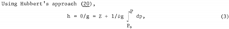
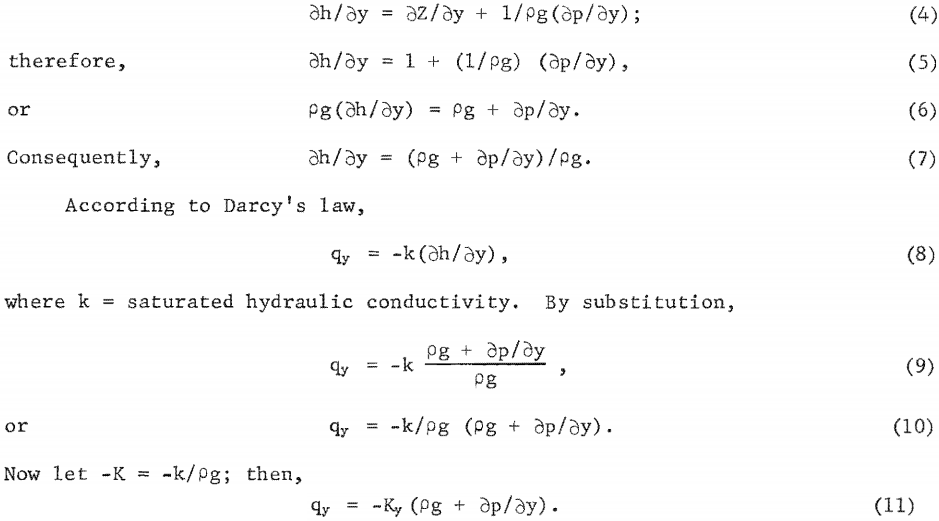
This expression can be derived in the manner shown in equations 3 through 16. The additional notation used consists of the following:

θ = fluid potential (L²/T²).
Z = elevation above a standard datum (L).
P = pressure at a point in the porous medium where θ is desired (M/LT²).
P0 = pressure at the standard datum (M/LT²).
k = saturated hydraulic conductivity (coefficient of permeability) (L/T).
qy = rate of flow in y direction (L/T).

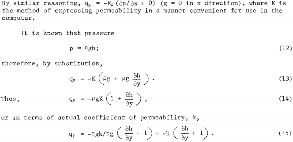
provided p and g are considered constant. Now, consider for example the potential gradient in the vertical direction (y direction);

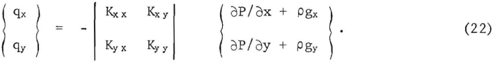
Consequently, if all nodal pressures are expressed in terms of hydrostatic head and if Pg = 1, then K (computer) can be replaced by k (measured). This practice was followed throughout the investigation. If program input pressures are in feet of water and if nodal coordinates are in feet, then q will have the same units as the input k units. Equation 2 can be expressed in matrix form as

where (q) is a matrix of the flow velocities, {k} is a matrix of the coefficients of permeability, P is the fluid pressure at a point {x}, and Pg is the gravitational term.

Directional Relationships: Theory and Application

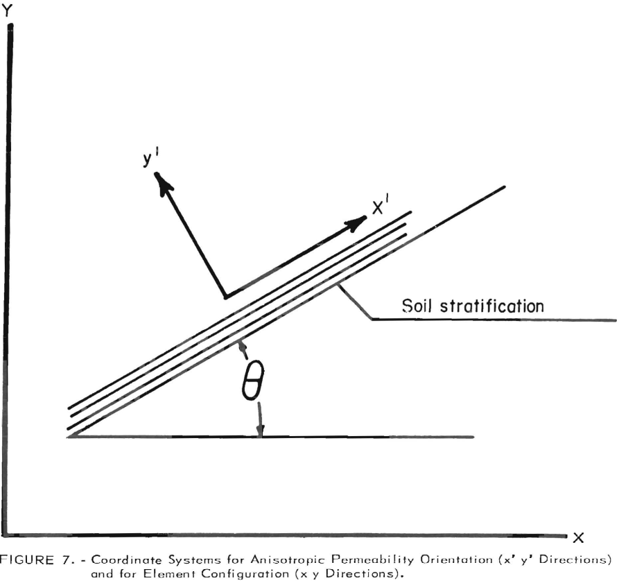
Because of testing limitations, k is measured parallel with and perpendicular to soil layering. Two sets of coordinates are required, designated x y and x’y’. (See fig. 7.) Directional permeabilities are specified in the x’y’ coordinate system as Kx’ and Ky ‘. The stratification angle is specified in the coordinate system x y.

Note that K must be measured in the field in x’y’ system.

Using standard transformation techniques (51), it can be shown that

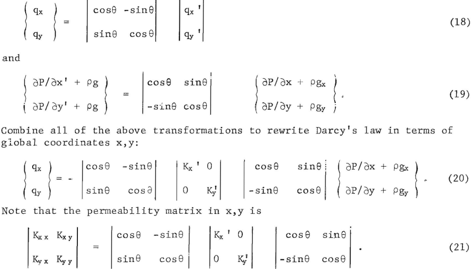
Therefore, the working equation in matrix form becomes

Linear Pressure Variations: Basic Assumptions

With Darcy’s law in the form of equation 22 and with the assumptions necessary for its use, it can be employed in flow analysis. However, an additional assumption is necessary: In each finite element (triangle) in the model the pressure varies linearly with the distance from nodes. Therefore, from equation 2, it can be seen that the fluid (water) velocities will be constant in time since the permeability and the gravity term pg are constant for any element.

Since the boundary node pressures are known in any problem under solution, it becomes advantageous to work in terms of node values. In any triangular element, the linear pressure variation can be expressed in terms of the pressures at the vertices i, j, and k of the triangle, these are called nodal pressures.

Derivation of Linear Pressure Distribution in Terms of Nodal Pressure

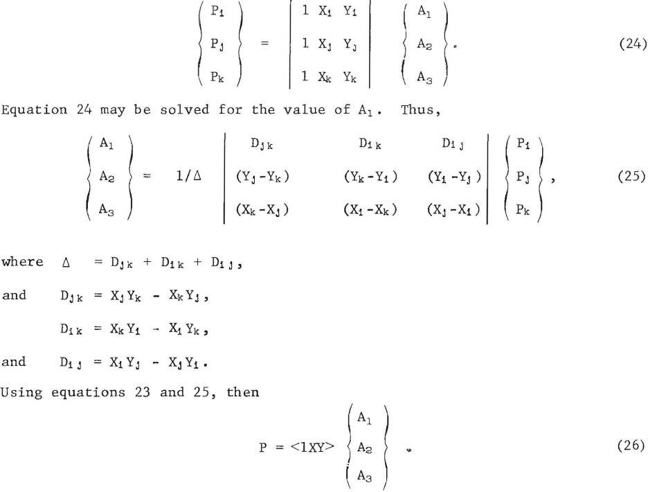
The following derivation is after Taylor. For a general linear spatial variation of pressure in a plane, the following applies:

P = A1 + A2X + A3Y……………………………………(23)

The constants A1, A2, and A3 can be expressed in terms of the nodal pressures located at the vertices i, j, and k, respectively, of a plane triangle by evaluating equation 23 at each node. Accordingly,

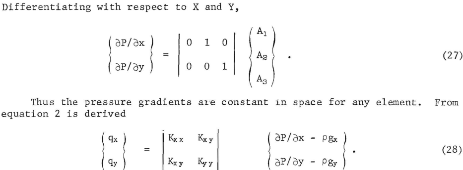
Consequently, for constant permeabilities {K} and gravitational term {pg}, the flow rates {q} will also be constant. Therefore, the flow problem is steady state, and the right-hand side of the continuity equation can subsequently be set equal to zero.

Continuity Equation

If no fluid is placed in or derived from storage in each element, then the continuity equation must be expressed for steady-state conditions; specifically, the flow into the region of study must equal the flow out of the region. If this concept is used on a single element of the region being studied and if a linear spatial-pressure distribution within the element is assumed, one can construct an approximate solution. Further, taking a large number of elements in the region of interest makes possible very accurate approximations.

A single element with nodal pressures, nodal volume rate of flow, element velocities, and element dimensions is portrayed in figure 8. The element velocities qx and qy, computed from the Darcy equation 2, are expressed in terms of the nodal pressures at the vertices i, j, and k, which are denoted by Pi, Pj, and Pk, respectively. Once qx and qy are known, equivalent nodal flows Q can be computed; that is,

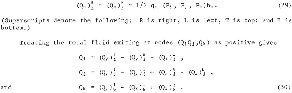
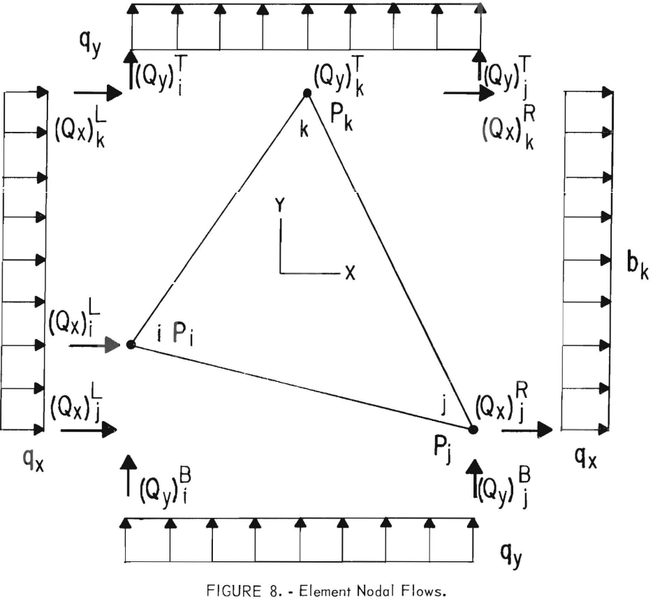
By considering each element connected to any node M, continuity of flow at the node is insured by

where m is the number of elements connected to node M and i is the particular element from which is computed. Computing equation 31 for each node in the finite element model requires a set of simultaneous algebraic equations in terms of the nodal pressures PM. (Recall that qx and qy are expressed for each element in terms of the element’s nodal pressures; consequently, each in equation 31 will also be in terms of the nodal pressures.) The algebraic equations were developed by considering each element in turn; the fact that certain nodal pressures are known and assigned was disregarded. For example, in figure 5 the pressures are known (or assumed) for all nodes located along the side boundaries. Before the algebraic equations are solved simultaneously, the equation for each node at which the pressure is known is modified to produce this pressure as the solution. The value of all other nodal pressures is obtained from the solution to the simultaneous equations. Once the pressure distribution is ascertained, the flow velocities in each element can be computed from Darcy’s equations. Further, if pressure distribution is known, then the potentials, or hydraulic head, can easily be calculated and the flow net derived.

Determination of Location of Free Water Surface

It should be recalled that the initial location of the free water surface was estimated, or assumed known, when the region of study (the flow region) was defined. In most real problems, the location is not known. Herein lies one of the main advantages of this particular numerical solution: With only minimal known boundary conditions, one can analyze an anisotropic flow system, as well as establish the locations of the phreatic surface.

In order to locate the free water surface, the investigator must be able to select the position of the surface that has both zero flow normal to it and zero atmospheric pressure on it. Using finite-element estimation, one should specify these two conditions at only the nodal points along the free surfaces. The final node location of the free water surface is not known beforehand.

The two foregoing conditions are specified for any node on the free surface as

P → 0 (where 0 is taken as atmospheric pressure) and q (normal to free surface) = 0.

The free water surface is finally located at those nodes where q = 0 and where P approaches 0.

It is not possible initially to specify correctly all three of the foregoing conditions because the node location at which the flow will be zero (and where the pressure will be atmospheric) is not known; therefore, the node location along the free surface must be asssumed. Further, because of the number of unknowns and equations to be solved, one must set either P = 0 or q = 0.

In this analysis q is always set equal to zero. Once so positioned, the initially located free surface nodes can be allowed to move until they reach points where P -» 0. This procedure provides the final location of the free surface nodes since all three conditions are satisfied (P → 0, q = 0, and free surface nodes are specified).

In Taylor’s program used here, all of the foregoing manipulations are performed on a digital computer; he identifies the program as FPM500. The original program has been modified in appendix A. This program has not been published; the source deck was obtained directly from Taylor.

Application of the Finite-Element Technique

Node Generation and Negative Areas

One of the requirements of the free surface model is that the free water surface must move up and down inside the geometry of the model. Since one cannot allow nodes to move across soil boundaries, the direction that the nodes move must be specified. In all models considered herein, the soil boundaries within the embankment parallel the slope of the face of the embankment. Consequently, in all models the nodes have been moved parallel to the slope of the embankment. In early models, long, slender triangles were used so that a negative area would not be developed as the free surface moved through the full dimensions of the embankment. In this manner the free surface would move from top to bottom. If a free surface node should cross another node, a negative area is produced, then further computation is canceled. Thus, restrictions govern how the free surface nodes can be placed in the elements developed. These problems can be eliminated by generating new nodes whenever it is suspected that movement of the free water surface may cause negative areas. Details of node generation are presented in appendix A.

Utilization of the Program Developed From the Darcian Theory

The user of this program should consider the following:

1. A thorough understanding of fluid mechanics and of soil mechanics is required if realistic boundary conditions are to be applied if true solutions to flow problems are to be derived from this technique. Erroneous boundary conditions may produce an apparently acceptable output, which may be completely in error and go undetected unless the boundary conditions are corrected or unless a check is made with field data.
2. One must understand the theory presented herein so that the basic units and the documentation presented in appendix A can be correctly applied.
3. Moreover, the user must have a graphical description of the geometry of the flow problem he is trying to interpret, and realistic parameters must be put into the program (along with the appropriate boundary conditions).
4. After considerable experience has been developed in element construction, then one can use the features built into the program for generating nodes, boundary conditions, and elements. They must be used with caution; however, they are essential, as well as timesaving, in building models.
5. Characteristics inherent in the theory cause problems at one exit node on the free surface. However, a finer mesh in this area (most conveniently achieved by node generation) will produce satisfactory results.
6. Input units and dimensions for the coordinate system and the fluid media used must be carefully and consistently chosen. Pressure must be expressed as head (length); permeability as a velocity (length/time); and unit flow as a velocity (length/time).
7. If the program is moved from one computer to another, care must be exercised to assure that the compilers and other accessory software of the computer are compatible with the program. A sample or check problem should be run. Further, it is advisable to run a problem to which the answer is known; for example, the Dupuit parabola may serve as a cross-check,
8. If at all possible, field data should be used to verify the solution (output) at various points throughout the mesh finite-element net.
9. If the output is to be effectively interpreted, it is necessary to have a plotter and its associated conversion program similar to the one used herein

Comparison of Dupuit Solution With Finite-Element Solution: An Example Problem

To provide greater acquaintance with the finite-element technique, a simple example is presented. The familiar Dupuit parabola is simulated (fig. 5). As portrayed here, the Dupuit parabola is based on the following two equations:

Q = K/2L (Ho² – Hi²)……………………………………(32)

and h2 = -2QX/K + Ho²………………………………..(33)

where Q = flow (L²/T),
h = height (L),
K = permeability (L/T),
L = length (L),
X = distance (L),
Ho = upstream water head (L),
and H1 = downstream water head (L)

The plot of the analytical phreatic surface is shown in figure 5. Because of certain assumptions on which the Dupuit parabola is based, the analytical location is only approximately correct; it must always be lower than the true surface. According to Sowers, the true phreatic surface must exit above the Dupuit analytical solution; it must also maintain equal potential drops across each unit length of the soil. The dotted line in figure 5 is a plot of the computer output as determined by program FPM500 of this report.
As expected, the finite-element answer does provide the true, higher phreatic surface with equal potential drops. Importantly, it should be noted here that the Dupuit analytical solution is valid only for isotropic, homogeneous conditions. If one needs greater versatility, such as anisotropic conditions, the Dupuit parabola cannot be utilized.

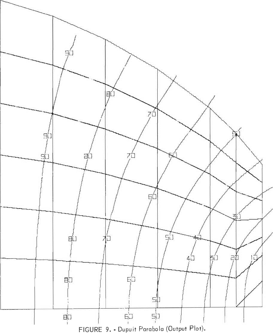
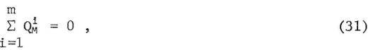
Figure 9 illustrates the equipotential lines for the model shown in figure 5, (See appendix C for the complete solution, including 14 iterations and the element flow quantities.) Not only does one develop the finite-element mesh with the plotter; he also uses it to contour the equipotential values and to obtain the final solution without any manual drafting. With complicated meshes it is advisable to plot the finite-element mesh on the computer prior to obtaining a solution to the flow equation; thus any error in mesh coordinates or element simulation can be detected. If one is purchasing computer time, this is standard practice. The mesh-plotting program was developed at the Bureau’s Spokane Mining Research Laboratory (SMRL), whereas the contouring program was developed by IBM.

The selection and utilization of a standard datum for equipotential line values can be controlled by specifying the potential references as indicated in the documentation in appendix B. The entire method of preselecting equipotential values is shown. With a contouring program, one can reproduce whatever contour value he desires. Spacing, grid size, and contour interval specification are well documented elsewhere. It should be noted, however, that, even with canned programs, considerable effort and time are required to fit them to an individual computer and to adjust the documentation to fit specific needs.

Finite-Element Models of Tailings Pond Embankments

Inhomogeneous Embankment on a Permeable Base With No Provision for Node Generation

A series of simple-to-complex tailings pond models will now be presented. Figure 10 shows a simple model of a simple mesh for an embankment on a permeable base. Provision for node generation is not included. The simple mesh structure is presented here for clarity. It consists of four soils, which would be common to a small tailings pond. In utilizing the finite-element program, one can specify various stratification, inclination, permeability, and location parameters for each soil. In fact, he may inadvertently introduce unplanned lenses.

Homogeneous Embankment on an Impermeable Base

Homogeneous and three-soil models were used to approximate a hypothetical tailings pond embankment. A three-soil model was constructed for an impermeable base material; a six-soil model was built for various base materials.

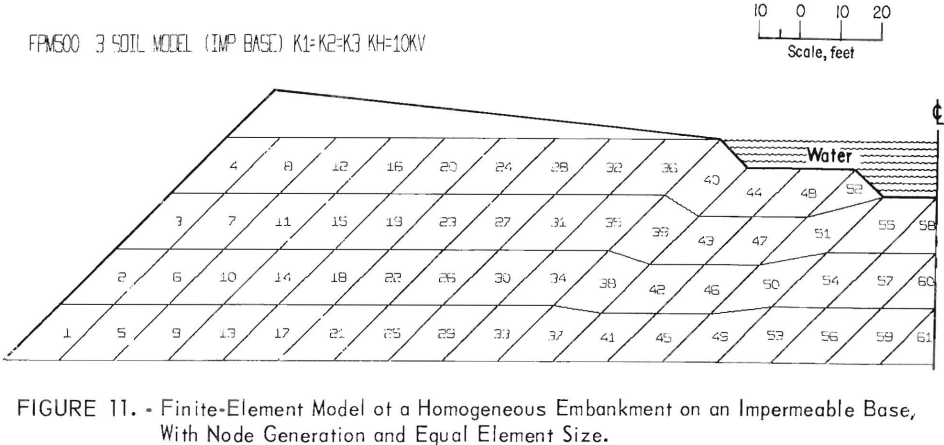
A model of a homogeneous embankment on an impermeable base was used (fig. 11) with node generation and boundary condition generation, but without reduction in element size at soil interfaces and at exit points. It was found that convergence was too slow and also that some “smoothing” effects were encountered at the interface.

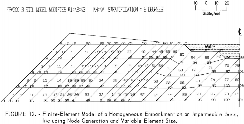
This experience led to the final models, which include node, boundary condition, and element generation within the program. By “stringing” these nodes and attaching them to the free surface which moves, regeneration is propagated with each iteration. Thus, no negative areas are produced; only the size of the element changes. If one inserts a high estimate of an input free surface (as indicated in fig. 12), the elements will be compressed, and more accurate solutions will be obtained.

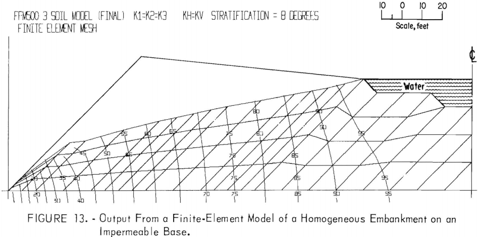
Figure 13 shows the potential distribution and phreatic surface for a homogeneous embankment on an impermeable base. As would be expected, equipotential lines approach the phreatic surface at equally spaced intervals. If a more accurate surface location at the exit point is desired, it could be obtained by increasing the number of elements near the exit surface.

Homogeneous, Anisotropic Embankment on an Impermeable Base

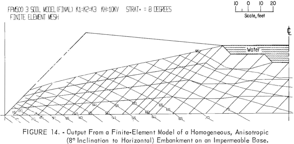
Figure 14 portrays the potential distribution and phreatic surface for a homogeneous embankment with anisotropic permeability, wherein the horizontal permeability is inclined at 8° to the horizontal X-axis. This configuration has been observed to be common in tailings pond embankments. In this case the exit point is higher than in the isotropic, but the remainder of the free surface is at the same location as shown in figure 13. Because Kh = 10Kv, the equipotential lines are inclined. Other runs were conducted with Kh ≤ 100Kv, but only slight changes in the location of the free surface occurred. The inclination of the equipotential lines becomes less as Kh → Kv .

This observation is most important because increasing Kh to 10Kv has in most earth dams a profound effect on the location of the free surface. The difference, of course, is caused by the location and inclination of the boundary-potential surface upstream from the dam (fig. 4). For tailings pond dams., the centerline, or the upgradient boundary of the flow region, is a flow line instead of an equipotential line.

Several experimental computer runs were made with the centerline an equipotential line. The high free surface was always obtained; it rose as Kh became greater than Kv.

Homogeneous, Anisotropic Embankment With Permeability Axes Horizontal and Vertical

Figure 15 portrays the phreatic surface and potential distribution for Kh = 10Kv, with the permeability axes horizontal and vertical. A comparison with figure 13 reveals that an 8° inclination of the anisotropic permeability

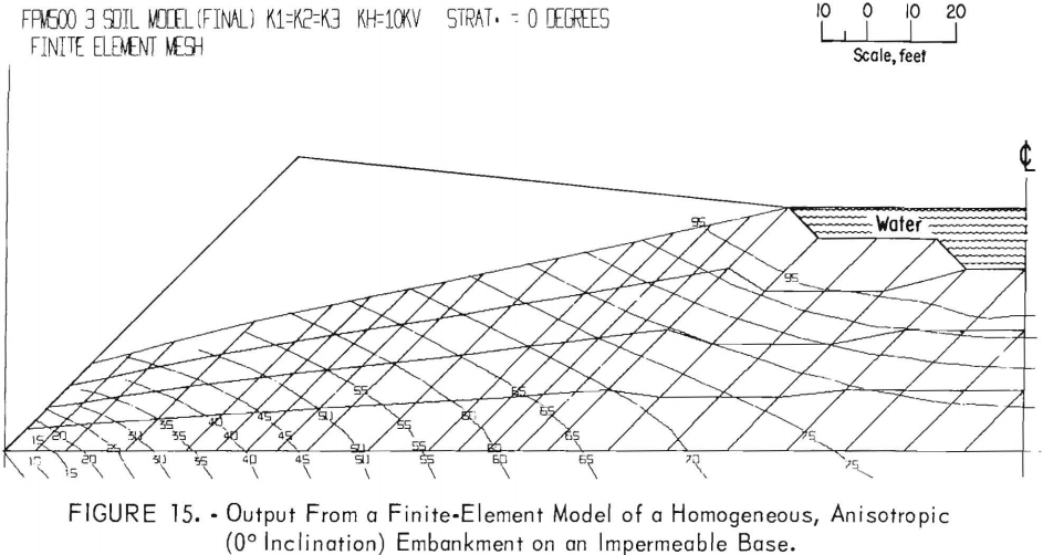
axes has a negligible effect on the free surface location. However, flow quantities are greater with a 0° inclination than with an 8° inclination.

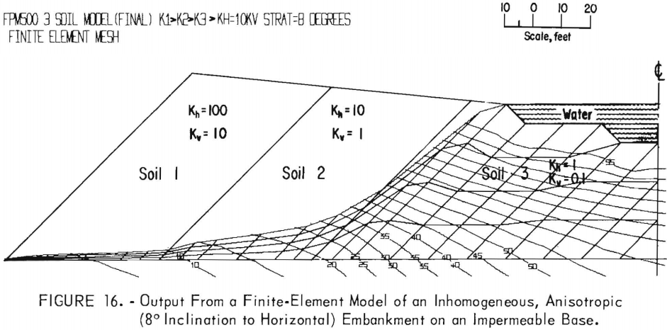
Inhomogeneous, Anisotropic Embankment With 8° Inclination of Permeability Axes

Presented in figure 16 are the phreatic surface and potential distribution for three soils, the horizontal and vertical permeabilities differing as shown in the figure. Anisotropic permeability axes are inclined at 8° with the horizontal. This arrangement of permeability has by far the most profound effect on the location of the free surface. The equipotential lines are much more closely spaced in the less permeable No. 3 soil. The phreatic surface acquires a pronounced concave configuration. In terms of slope stability, this permeability configuration would offer ideal conditions.

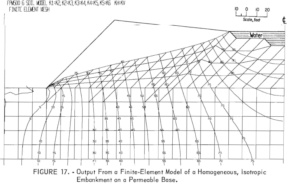
Homogeneous, Isotropic Embankment on a Permeable Base

Figure 17 presents the phreatic surface and potential distribution for a homogeneous embankment on a base having the same permeability as the embankment. As would be expected, the free surface is lower than the phreatic surface in a similar embankment over an impermeable base.

Homogeneous, Isotropic Embankment on a Base With Permeability Equal to 0.1 That of the Embankment

Figure 18 illustrates the phreatic surface and potential distribution for an embankment with an isotropic permeability 10 times that of the base. As anticipated, the free surface is higher in the embankment. The equipotential

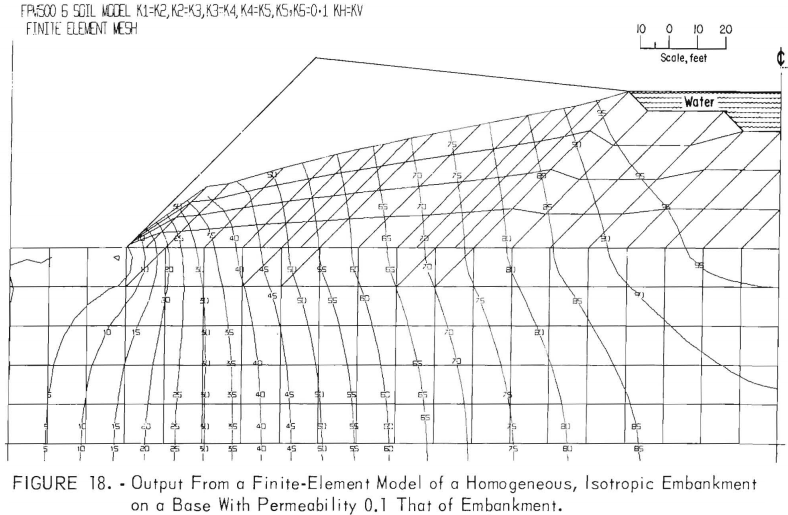
lines are refracted as they cross the permeability boundary at the base of the embankment. The refraction increases discharge at the toe of the embankment.

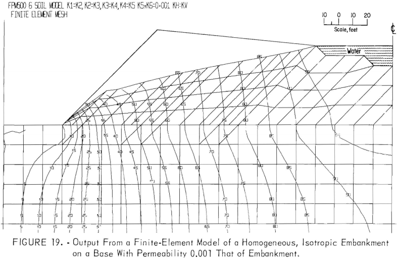
Homogeneous, Isotropic Embankment on a Base With Permeability Equal to 0.001 that of the Embankment

Shown in figure 19 are phreatic surface and potential distribution for an embankment with an isotropic permeability 1,000 times that of the base. Only a slight change from the phreatic surface in figure 7 occurs. This result supports the widely used assumption that a base can be considered impermeable, with but slight error introduced, if the base is in fact less permeable than the embankment.

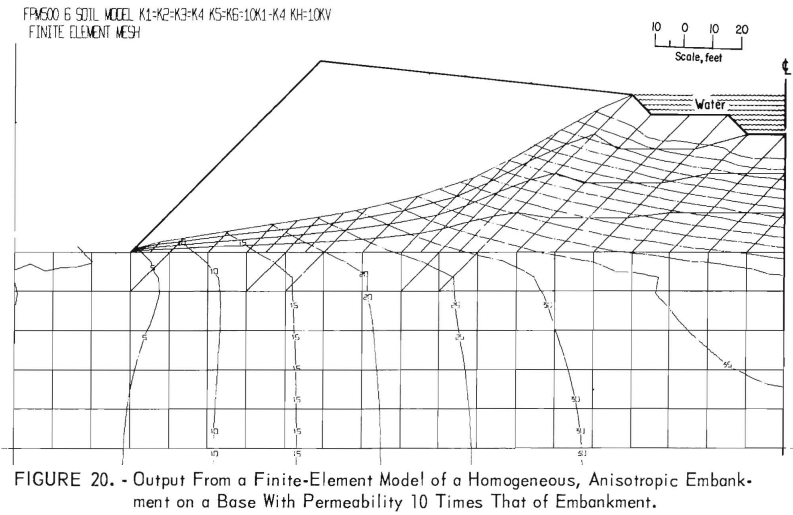
Homogeneous, Anisotropic Embankment With Permeability of Base 10 Times Greater than that of the Embankment

Figure 20 portrays the phreatic surface and potential distribution resulting from a base 10 times greater than that of the embankment. As expected here, the phreatic surface is considerably lower than that of the less permeable base.

Analysis of Parameters for a Tailings Pond Model

Selection of Field Site and Parameters to be Examined

Field work conducted by the Bureau’s Spokane Mining Research Laboratory (SMRL) throughout the United States in the past 2 years provided the data on which the models included herein were developed. The writers collected numerous soil samples for density and permeability analysis. At this writing, data are being assembled for verification of some recent computer runs. In addition, the hydraulic backfill program at SMRL has included numerous tests on percolation and permeability of various hydraulic fills (3, 30, 46). These values also were considered during development of the finite-element model.

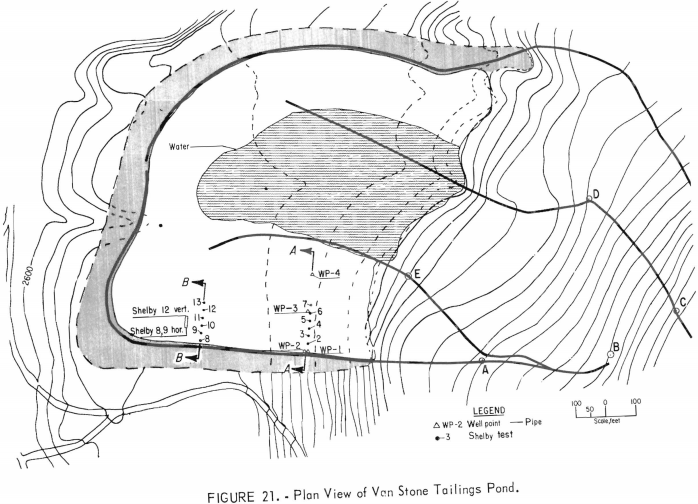
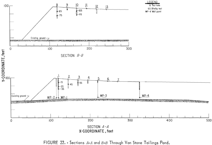
Because of the convenient location and size of the Van Stone pond, which is owned and operated by the American Smelting and Refining Company (ASARCO), it was chosen for the collection of detailed field data to insert into a finite-element model. Figure 21 portrays the plan view of the Van Stone tailings pond and the general disposal system. This is a lead-zinc operation producing approximately standard-grind mill tailings. The pond has a peripheral discharge system, and water is decanted from the center portion. Because of intermittent winter and summer operations, ideal stratification is not obtained. During freezing weather the coarse fraction is discharged in the center of the pond, and some discontinuities in the lens formation and in stratification of the layers result. Figure 22 shows a section through the pond for lines A-A and B-B. This pond also served as a testing ground for our field equipment and testing procedures.

Field Instrumentation and Testing at the Van Stone Pond

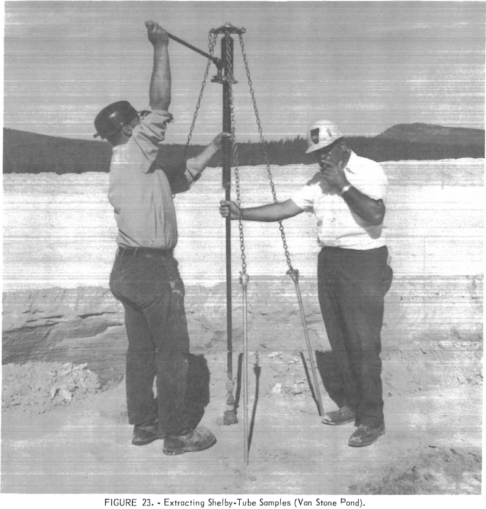
After an examination of several sections of the pond, it was concluded that the most representative section would be obtained as delineated along the line A-A in figures 21 and 22. An auxiliary section along B-B was also selected to analyze variation in grain-size sampling. Each line and the pond were surveyed so that maps could be constructed. The regional contouring was obtained from ASARCO. Shelby-tube samples were extracted along line A-A at predetermined intervals, as shown on the plan map. Since one can obtain Shelby-tube samples only from the vertical direction at depth, the horizontal permeability at depth had to be correlated with near-surface Shelby-tube samples extracted horizontally. A tractor was moved to the site; and, in order to obtain horizontal samples, a 6-foot trench approximately 50 feet long was excavated. Figure 23 shows a portion of the upper end of this trench. Note the stratification of the layering in the exposed embankment in the left side of the figure. The figure also illustrates the technique of forcing the Shelby tube into the tailings with the hydraulic jack and the power-pole anchors. This jacking procedure was utilized at depth, the samples being taken at 5-foot intervals. A hand auger and a gin pole were used to remove the material between the intervals from which the Shelby tubes were extracted. Our earlier investigation verified that we could obtain both permeability and density from the Shelby-tube samples.

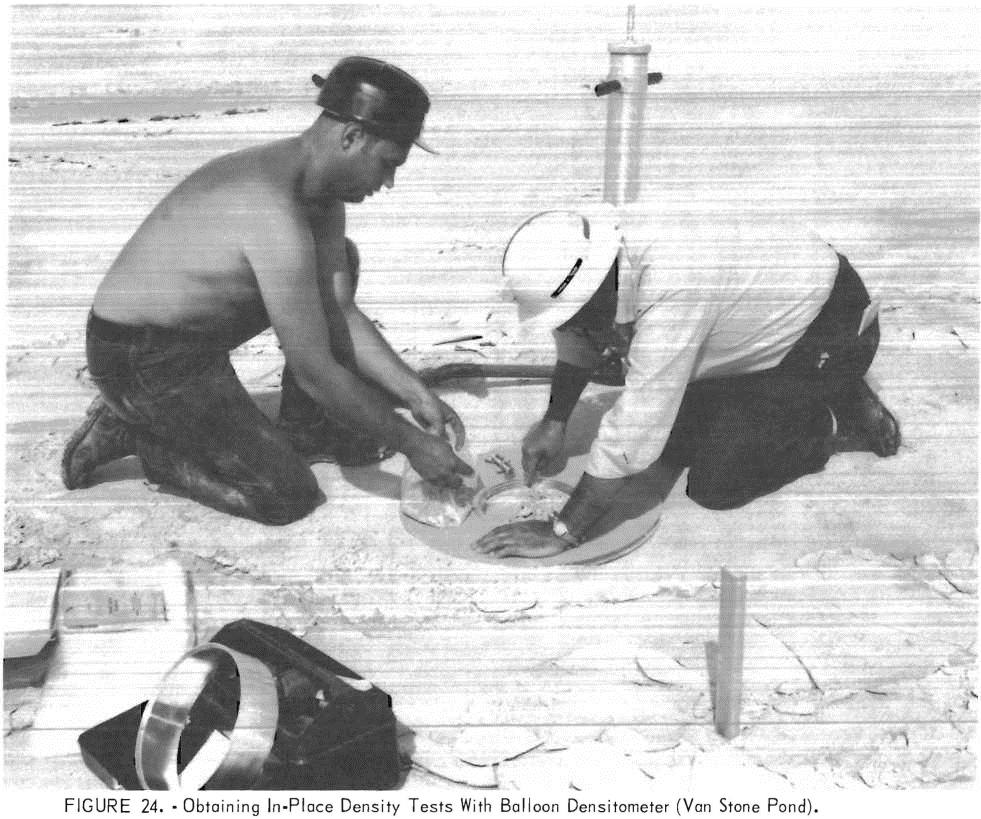
Both to facilitate comparison with other ponds that we had tested throughout the country and to secure a cross-check on the Shelby tubes, a standard balloon densitometer was utilized for sampling at and near the surface (fig. 24). This device measures the volume of the hole remaining after the soil is extracted and saved for weighing. Balloon-densitometer samples were obtained near the surface and also in the trench.

Results of Laboratory Tests on Samples Obtained from the Field

Since stratification consisted of thin varves, it was possible to conduct the laboratory permeameter tests without a breakdown of the individual layers in a Shelby tube, as would have occurred had the stratification been other than varved. All of the tests were conducted in the apparatus pictured in figure 25, which is a constant-head permeameter. Because each tube was forced into the varved soil either in a vertical or horizontal direction, directional permeability values could be derived from the appropriate orientation. Figure 26 shows a closeup view of the fabrication of the O-rings and the feed pipes that were built at the Bureau of Mines in Spokane. No seepage about the O-rings was observed, although this contingency cannot be eliminated. The two major weaknesses of this type of test are the disturbing of the sample and the possible percolation of water along the tube wall. One major advantage is that, once obtained, the soil is never removed from the sample container; consequently, repetitive tests can be conducted at any time.

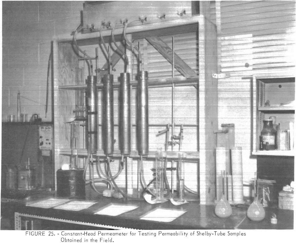
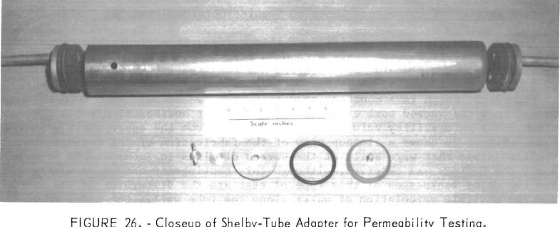
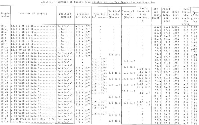
Table 1 presents values of parameters obtained from Shelby-tube samples,, The series of values for permeability from samples taken demonstrate the value of the Shelby tube for easily obtaining undisturbed, oriented, permeability tests on fine sands. As presumed the results reveal a decreased permeability with depth as well as a definite correlation between the effective grain size and the permeability. Sample VS-11 is especially interesting; it shows a low permeability and density. This relationship reflects the presence of clay slimes in this area of the tailings pond.

The main purpose of collecting the surface samples was to determine the ratio between horizontal and vertical permeability. Column 6 in table 1 shows this ratio for samples obtained from points as close as possible to each other. The tests that yielded these values were conducted in the laboratory by injecting water through the top of the vertically oriented tube. These data point out that the average horizontal permeability is about 5 times as great as the vertical. It must be recognized here that, although the samples were taken from the same location, an occasional thin horizontal layer of slimes or coarse sand picked up in the horizontal sample may have had a significant influence on the effective size, but not upon the permeability. It is theorized that this problem is responsible for the range of ratios.

Column 7 is another comparison of horizontal and vertical permeabilities; here the results were obtained by inverting the tubes in the laboratory and injecting the water through the bottom. Originally it was believed that the effect of entrapped air might be thus minimized. With the exception of VS-34 which was disturbed while inverting and should be neglected the average ratios show the horizontal permeability to be about 6 times the vertical. The effect of injection from top and bottom appears to be similar. The ratio of permeabilities obtained from inverted and noninverted samples averaged about 1.15, indicating the very slight effect of gas blockage

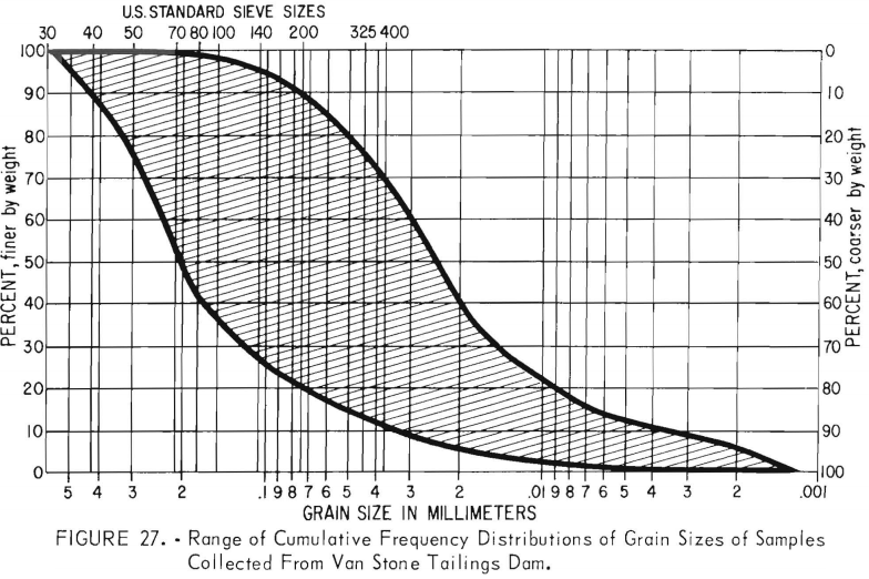
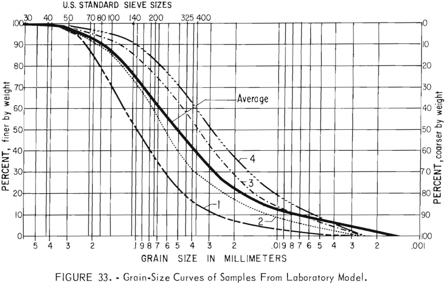
Figure 27 presents the range of the cumulative frequency distribution of the grain sizes observed in all Shelby-tube samples collected from the Van Stone pond embankment.

Laboratory Model of Embankment

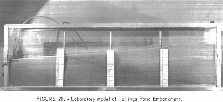
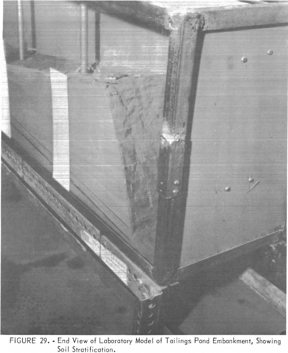
The complicated structure of tailings disposal used at the Van Stone mine, caused by peripheral discharge in the summer and interior discharge in the winter, prompted construction of a pond model in the lab. For this model a tailings sample was obtained at the mine site and transported to the laboratory, where it was slurried to the same density as when discharged at the mine. The slurried sample was then poured into the container, as illustrated in figure 28. As is normally done in a tailings pond, the pours were consecutive. Figure 29 indicates the resulting varves. The anticipated segregation and distribution of the coarses and fines were also simulated. After the pours had been completed, the simulated pond was allowed to drain and dry so that samples could be extracted for laboratory testing. Figure 29 shows details of the sample layering as well as the inclination of the layers.

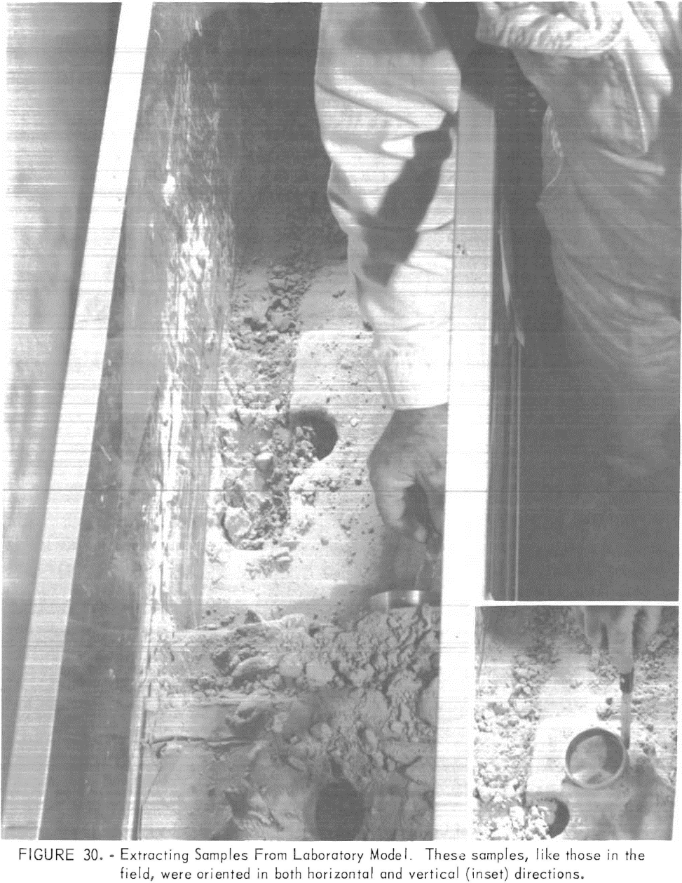
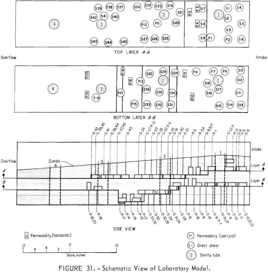
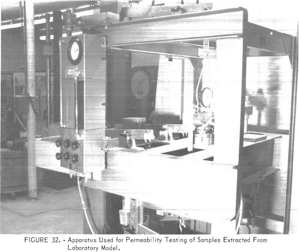
Samples were extracted with a thin-wall tube sampler to obtain the average density and grain size throughout the zone. Later, a series of samples was obtained with a circular trimmer ring for permeability and direct-shear testing. These samples, like those in the field, were oriented in both horizontal and vertical directions (fig. 30). The samples were extracted in the locations shown in figure 31 and tested with the apparatus shown in figure 32.

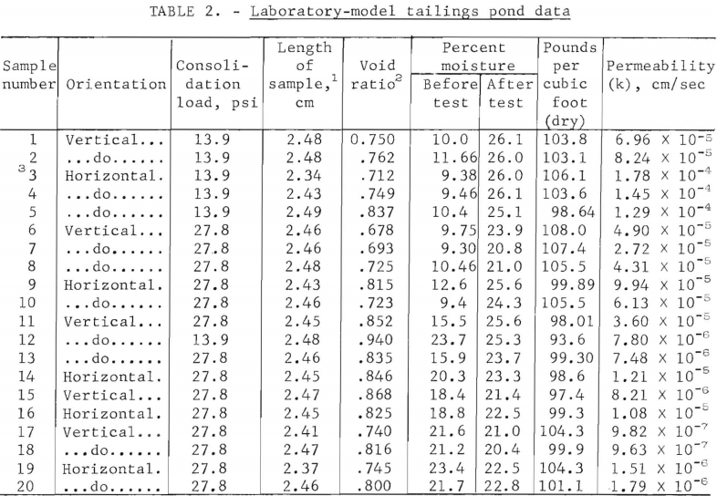
A summary of the grain-size distribution is given in figure 33, and the permeability values obtained in this model are entered in table 2.

As stated in the “Introduction,” one of the purposes of this model study was to develop the values of parameters that are valid for the physical modeling of tailings pond embankments and to examine the feasibility of a finite-element model for interpretation of the fluid flow characteristics within the embankments. Field data were obtained to develop experiential methods of application in the field, but at this stage, it was not the intent to develop final numbers for the finite-element model rather to amass sufficient data for its interpretation and realistic application.

Table 2 shows that as one proceeds inward from the face of the embankment some consolidation takes place. This consolidation is highly operative in

samples 16, 17, and 18 obtained from a slime area. Therefore, any finite-element model should consider the change in permeability of a soil in the slime area to simulate this effect.

Permeability decreases inward from the face of the embankment. The ratio Kh/Kv is not as great in the laboratory model as that observed in the field. However, a comparison of the laboratory and field permeability of all values could not be made because it was impossible to sample the intermediate and slime zones in the field. Analyses of lab and field samples obtained from the portion of the embankment near the face do compare favorably. (See tables 1 and 2.)

Finite-Element Model Applied To The

Van Stone Tailings Pond Embankment

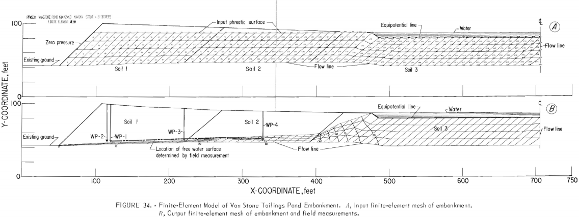
Figure 34A portrays the finally selected model of the Van Stone tailings pond embankment. The geometry of the soils having different permeabilities is based on the data in tables 1 and 2, on the grain-size curves presented in figures 27 and 33, and on field and laboratory observations. Also shown in figure 34 is the hydraulic character of each boundary. Comparison of model outputs with field water-level measurements revealed early that realistic results could be obtained from the model only if the vertical portion of the upgradient boundary were treated as a flow line, in a manner similar to that used by Hantush. Early attempts to treat the upper boundary as an equipotential line, as would be the case if the embankment were similar to an earth dam, yielded results that could not be validated by field data. A more complicated six-soil model was studied by Kealy, which takes into consideration the consolidation of the lower soil layers, because density and permeability change as consolidation increases with the height of the dam.

More consolidation occurs in the slime portion than in the other soils. In addition, percolation of the fines into the very top substratum, which would change its premeability characteristics, is represented in the six-soil model sighted in references 25 and 27.

For analysis of the Van Stone tailings pond, the extracted numbers are as follows:

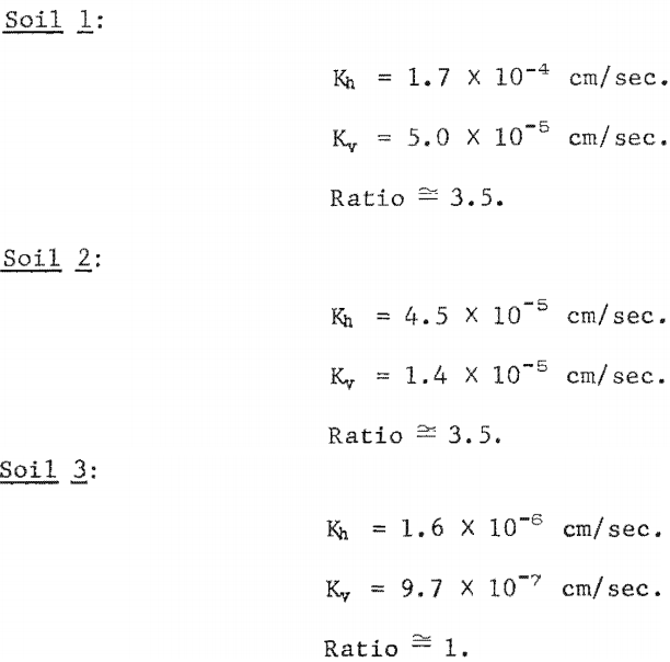
Much more sample testing is required before statistical realiability can be assigned to these numbers; however, they constitute all available field data.

Once the soil boundaries have been defined and the location of the water body above the slime area has been inserted, then a finite-element mesh can be drawn over the geometry of the pond. Also inserted is the estimated location of the phreatic surface, which later will be determined accurately by the program. After construction of the elements, one must assign values to the angles of stratification of the layers and also to the permeability of the soils in both the horizontal and vertical directions. When so done, the known boundary conditions can be applied to the elemental nodes.

In this model, the pressures directly below the free water surface nodes 200, 205, 210, 310, in the center of the pond, are known and assigned. Their values are obtained simply by P = pgh. Also, assuming that the water table occurs at ground level on the downstream side of the embankment, the pressures at node 1 can be assigned zero (which in this case is treated as atmospheric pressure). The boundary condition along the downstream face nodes 1, 2, 3, and 4 is expressed as zero pressure. The third boundary condition consists of an impervious base along nodes 1, 6, 11, 320.

Following the establishment of these criteria, the data can be keypunched. Each node is punched by its coordinate; each element is described by the nodal points encompassing it. After these operations and after the control cards have been coded (as shown in the documentation in appendix A), a solution can be obtained. The output free water surface for the model in figure 34A is shown in figure 34B.

In addition to the phreatic surface predicted by the model, the phreatic surface as determined from water levels in the embankment is indicated in figure 34B. The equipotential lines predicted by the model are also shown. The measured phreatic surface was derived from the average of piezometer water- level readings taken over a 12-week period early in 1970. Figure 34B reveals that the measured phreatic surface is slightly different from the one predicted by the model, particularly at the downgradient end of the flow system. This slight discrepancy appears because we are unable to specify precisely the location of the boundaries between soils 1, 2, and 3. It is possible, but perhaps unrealistic, to juggle the positions of these boundaries on the data and field observations.. The phreatic surface predicted by the model is sufficiently close to the true phreatic surface to serve any of the purposes for which it was intended.

Appendix D provides a complete listing of the input nodal locations, material boundaries, material property values, and a listing of the final output iteration, which is No. 25.

The phreatic surface shown in figure 34B results in a factor of safety of 1.4 for the embankment slope shown. If the safety factor for the embankment shown is calculated on the basis of a Dupuit parabola, the value becomes 1.2. Consequently, it is essential that, when calculating their effect on slope stability, tailings pond embankments not be viewed as having hydraulic characteristics similar to those of an earth dam.

Conclusions

Based on computer output, a search of literature, and observations of tailings ponds, the following conclusions are drawn:

1. The finite-element technique will undoubtedly be the most useful available tool for analyzing seepage through porous media, both from structural and environmental viewpoints. The program presented herein can best be used if node, element, and boundary-condition generations are used. The element size should be reduced at the interface of two soils and at the exit points in any finite-element model, because convergence and accuracy can be strongly affected.
2. Tailings pond embankments do not have the same seepage characteristics as earth dams, primarily because the centerline (fig. 4A) is a flow line rather than an equipotential line.
3. The 8° inclination of tailings-sand stratification, which is common, has little influence on the location of the phreatic surface.
4. The horizontal-to-vertical permeability ratio is not nearly as significant in tailings pond embankments as it is in earth dams. This fact is due primarily to the difference in the location and inclination of the equipotential line at the upstream boundary within the two structures. The condition noted under conclusion 2 also aids in restricting the variation of the surface with permeability. Kh = 10Kv will not move the phreatic surface line appreciably, except at the last node adjacent to the exit point on the downstream face.
5. By far the most significant factor in determining the location of the free surface is relative permeability progressing from the downstream face to the interior of the pond. Slight changes in the relative permeability make large changes in the location of the free surface.
6. Changing the base-soil permeability from 0.1 that of the embankment to 0.001 that of the embankment has little effect on the location of the free surface. Therefore, if the permeability of the base is less than that of the embankment, the common assumption of an impervious base is valid. It should be noted, however, that a very high permeability base relative to the embankment will be influential.
7. A comparison of the field and lab-model data indicates that it may be possible to model a pond prior to its construction.
8. The finite-element solution to the Van Stone tailings pond does compare favorably with measurements conducted in the field. It thus confirms the practicability of using this technique for designing tailings pond embankments.

Additional research will include instrumentation and the sampling techniques to obtain realistic values of the parameters used as input into the computer program. More research will also be required in environmental control relative to ion exchange; that is, numerous ions in the waste water can be, and are being, absorbed as the water moves from the free surface into the substrata through the pond. Presently, essentially nothing is known about adsorption characteristics of these materials.

It should be pointed out also that the finite-element technique can be applied to prediction of the phreatic surface and flow of water through open pit dumps and in underground mining installations, as well as to tailings ponds and embankments. Control of mine water, both from a structural and environmental viewpoint, underground and in open pits, has been sadly neglected to date. As of late forcefully manifested, public opinion will no longer permit such negligence. Refined techniques such as finite-element analysis are available and must be utilized for the examination of such problems.