Description

75 mm (3 inch) diameter cyclone

50 mm (2 inch) diameter cyclone

25 mm (1 inch) diameter cyclone

Hydrocyclone Size Compared – 3″, 2″ and 1″ (75mm, 50mm, 25mm)

Experimental Procedure

For the experimental work, two conventional hydrocyclones were selected. Both manufactured by R. Mozley Ltd., these were a 50mm (2″) and a 25mm (1″) standard units. A complete range of vortex finders and spigots was used. Each hydrocyclone can be mounted in the Hydrocyclone Test Rig, which consists of a 40 1 sump, a slurry pump, a pressure gauge (0-100 psi) and a by-pass valve. Details of the Test Rig are shown in Fig. 1.

For the laboratory circuit, a timed, simultaneous sample collection system was available. Products and feed samples were weighed, sampled for size analysis before being dried and reweighed. All wet sizing was completed using a sieve shaking device (Gilson). With a single density feed material, these measurements enabled a complete flow and size mass balance to be computed. Feed size measurements were also compared with reconstituted values to verify the accuracy of the system.

Two test materials were selected. These were copper flotation tailings (density of 2.77 t/m³) and copper flotation concentrates (density of 4.44 t/m³). A summary of the test conditions is given in Table 1.

Experimental Results Analysis

The results are presented and analysed on the basis of capacity, water split, partition curve and corrected cut point (d50,c).

Capacity

Four different equations were tested in terms of their suitability for the prediction of the small diameter hydrocyclones capacity. These were those of Lynch and Rao, Bradley and two new equations proposed by the author.

The Lynch and Rao equation was tested in three different ways: (a) Two parameters with the values given by Lynch (A1 and A2), estimating K1; (b) Estimating all the parameters; and (c) Estimating K1 and A2, with A1 fixed in the value given by Lynch. With all the equations (for all data sets) the correlations are not good enough. Considering the standard deviation, the number of parameters, the predictive capability (simulation) and the correlation, the best equation was selected. This was the Lynch and Rao equation (Eq. 1), in which A1 has a fixed value given by Lynch of 0.5. The correlation for one of the data sets is shown in Fig. 2.

where:
K1 = Parameter, estimated for each set of data.
A1 = Fixed parameter = 0.5, for all data sets.
A2 = Parameter, estimated for each set of data.

Water Split

Three different water split equations were tested. These were those of Lynch and Rao, Brookes and a new equation proposed by one of the authors. The testing was done using the first two data sets, those with copper flotation tailings.

The Lynch and Rao equation was tested in two different ways: (a) Two parameters with the values given by Lynch (A1 and A2), estimating K3; and (b) Estimating all the parameters.

Considering the standard deviation, the number of parameters, the predictive capability (simulation) and the correlation, the best equation was selected. This was the new equation (Eq. 2), followed closely by the Lynch and Rao equation, with all the parameters estimated (Eq. 3). The correlations of both equation, for one of the data sets, is shown in Fig. 3. If those data corresponding to unrealistic water split values (greater than 0.5) are deleted, then both equations are comparables.

where:

K3, B1 and B2 = Parameters estimated for each set of data.

Partition Curve

For each one of the 74 tests, the partition curves (normal, corrected and reduced) were determined. The reduced partition values, for all the tests corresponding to a single ore, were plotted in a unic diagram presented in Fig. 4. It is possible to appreciate that a certain dispersion does exist, but also that most points are concentrated in what seems to be an average partition curve which is shown, in the figure, with a continuous line.

To represent the partition curves, the two more common efficiency equations were tested: Lynch and Rao and Plitt. The quality of both approaches are equivalent. The data processing using the Plitt model has been done and will be presented somewhere else. The data, shown in Fig. 4, corresponding to the tests (the first two data sets) where copper flotation tailings was used, were analysed and presented here using the Lynch and Rao approach.

The Lynch and Rao efficiency equation is represented as follows:

where α is a parameter that represents the separation sharpness, related with the imperfection “I” (Ep/d50,c = [(d75 – d25)/2]/d50,c), through the following equation:

The equation 5 is presented in Fig. 5, in a continuous line, together with the α and I values for the tests considered.

In Fig. 4 three different curves are shown. The average one (in continuous line) was calculated using a standard fitting method, considering all the experimental data above mentioned. The other two curves were calculated to isolate an area around the average curve with 90% of the experimental values. The α values, corresponding to the three curves, are:

-αm = 3.9(I = 0.27), for the average curve,
-αmin – 2.0(I = 0.47),
-αmax = 12.0 (I = 0.09).

Most of the experimental results (63% of those with the 2″ cyclone) have a values between 3 and 5 (0.34 > I > 0.21) and are well represented by the average curve. Most of the values out of limits correspond to tests with unusual operational conditions, for example with Apexs too small (producing roping) or too big (producing short circuits too high).

Corrected Cut Point d50,c

The d50,c equations tested were those of Lynch and Rao, Rouse, Plitt and a new equation proposed by one of the authors. The testing was done using the first two data sets, those with copper flotation tailings.

The Lynch and Rao equation was tested in two different ways: (a) Four parameters with the values given by Lynch (M1, M2, M3 and M4), estimating K2; and (b) Estimating all the parameters.

Considering the standard deviation, the number of parameters, the predictive capability (simulation) and the correlation, the best equation was selected. This was the Plitt equation (Eq. 6). The correlations of all the equations are presented in Table 2. The correlation curve of the Plitt equation, for one of the data sets, is shown in Fig. 6.

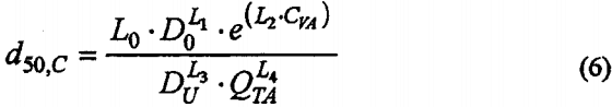
where:

L0, L1, L2, L3 and L4 = Parameters estimated for each set of data.

Conclusions

The present study has provided some useful information on the modelling of small diameter hydrocyclones.

1. The results show, in some aspects, coherency with what is already known about larger cyclones. The suitability of existing empirical models has been checked and their accuracy compared.
2. Modifications of the existing models equations are proposed, improving their predictive capability for the small cyclones performance.
3. All the capacity equations tested have, with the experimental data, correlations not good enough. The best one was a slightly modified Lynch & Rao equation.
4. A new water split equation was proposed. This equation shows, for those tests with copper flotation tailings, a better predictive capability than the other equations tested. However, a slightly modified Lynch & Rao equation, follows closely and if those data corresponding to industrially unrealistic water split values (greater than 0.5) are deleted, then both equations are absolutely comparables.
5. With respect to the partition curve, the Lynch and Rao approach was analysed. Most of the experimental results are well represented by the average curve. However, the Lynch assumption about a being only a function on solid characteristics and independent of hydrocyclone geometry and operation conditions, is not in accordance with the experimental data presented here. The experimental results show that some of the hydrocyclone dimensions (specially the Apex diameter) and also (but not as much) of the operation conditions, have influence on α.
6. The best of the d50,c equations tested, using those data sets with copper flotation tailings, was the Plitt equation, which shows a quite good correlation and predictive capability.
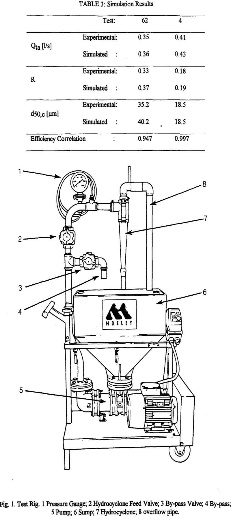
7. Simulation testing shows that the predictive capability of the model (the four selected equations) is adequate for the description of small cyclones performance.

In some respects this investigation has produced new questions. Clearly, more work needs to be done in this area to solve them. Until these questions are answered, the design and analysis of engineering problems, related with small diameter hydrocyclones, will have to rely only on good judgement.