The limitations that ore reserve estimators have faced in the past while trying to estimate recoverable reserves stem from different aspects. There are several factors that curtail the effectiveness of the “traditional” geostatistical models:

• A variogram model is required to derive the VCF; it is well-known that the VCF value itself is greatly influenced by the nugget effect of the variogram model used; the nugget effect of any variogram model is in turn very sensitive to trimming (or capping) the high grade composites from the database. This has a strong impact on the VCF used (Rossi and Parker, 1993a), particularly for gold-type distributions.
• The geometry of the SMU. VCFs are calculated based on a regular-shaped SMU. For example, a gold mine in northeastern Nevada (Douglas et al., 1994) used approximately a 5mx10m or 10mx10m “nominal” SMU size. In fact, mining practices are such that grade control panels will rarely match the “nominal” size and shape of the SMU. During mining, blast patterns and grade control panels do not resemble the planned SMU size and shape. It is discouraging to chase the parameters of an illusory and evasive SMU distribution, only to find out that such SMU does not approximate actual practices!
• Another major limitation is the difficulty in estimating “local” minable reserves. For example, they could be based on mining phases, or monthly productions in the early years of a deposit at advanced feasibility level development. Attempts to estimate recoverable and minable reserves locally, based on the geostatistical models mentioned, have proven dangerous. This is particularly true in the absence of production data use to fine-tune the output predictions.
• Other correction models are based on stringent Gaussian assumptions, such as multiGaussian kriging (Verly, 1983) and disjunctive kriging (Matheron, 1975a). and are not often used at operating mines because of their complexity. Also, the “lognormal shortcut” (David et al., 1977), developed originally for porphyry copper deposits, has produced biased results when dealing with highly skewed distributions (Rossi et al. 1993a).

Two recent papers from the previous SME conference relate to this discussion, although within a different context in one case (Davis. 1997), and exclusively for recoverable reserves in the other.

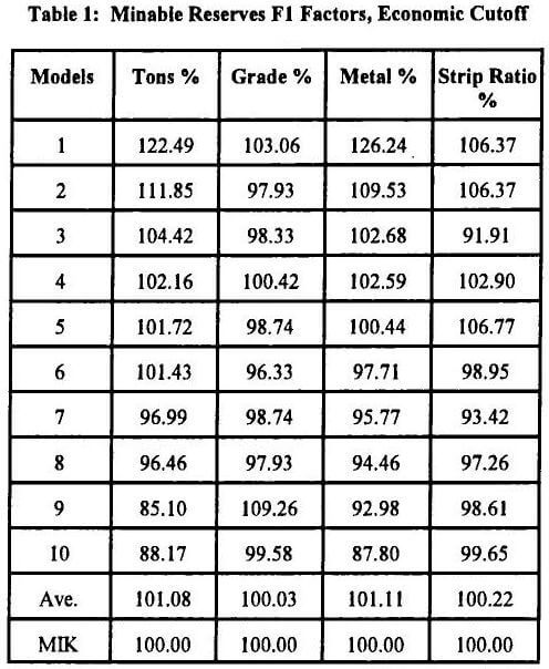
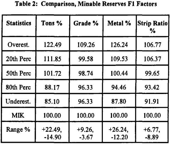
A more general procedure was recommended in Rossi et al., (1993b), involving two sets of reconciliations, evaluated based on the F1 and F2 factors mentioned in the abstract section. These factors measure the prediction performance, both in tonnage and grade, of the long-term block model with respect to the grade control model (TF1 and GF1), and the grade control model with respect to what has actually been achieved as head tonnages or grades (TF2 and GF2). The F1 and F2 factors are then defined as follows:

F1 = Long-term Block Model/Grade Control Model

F2 = Grade Control Model/Mill Feed

From these F1 and F2 factors, the performance of the long-term model against actual production data can be measured. This is called an F3 factor, and is simply the product of the F1 and F2 products: F3= F1 x F2.

An important and often forgotten (by geologists and ore reserve estimators) “F” factor is the one that would correspond for the planned strip ratio; a comparison of the strip ratio resulting from the block model with the strip ratios resulting from the simulations may be a very useful mine planning tool.

A single conditional simulation (“ground-truth”) is involved in the method outlined, as well as a grade control model and a long-term recoverable reserves model. By itself, this method avoids the caveats mentioned above for more “traditional” methods and does not require defining an SMU. However, it falls short of allowing a full description of the uncertainty involved in the long-term mine plan model, including confidence intervals on a month by month and/or phase by phase basis. Only a full set of conditional simulations can provide this.

Conditional Simulations

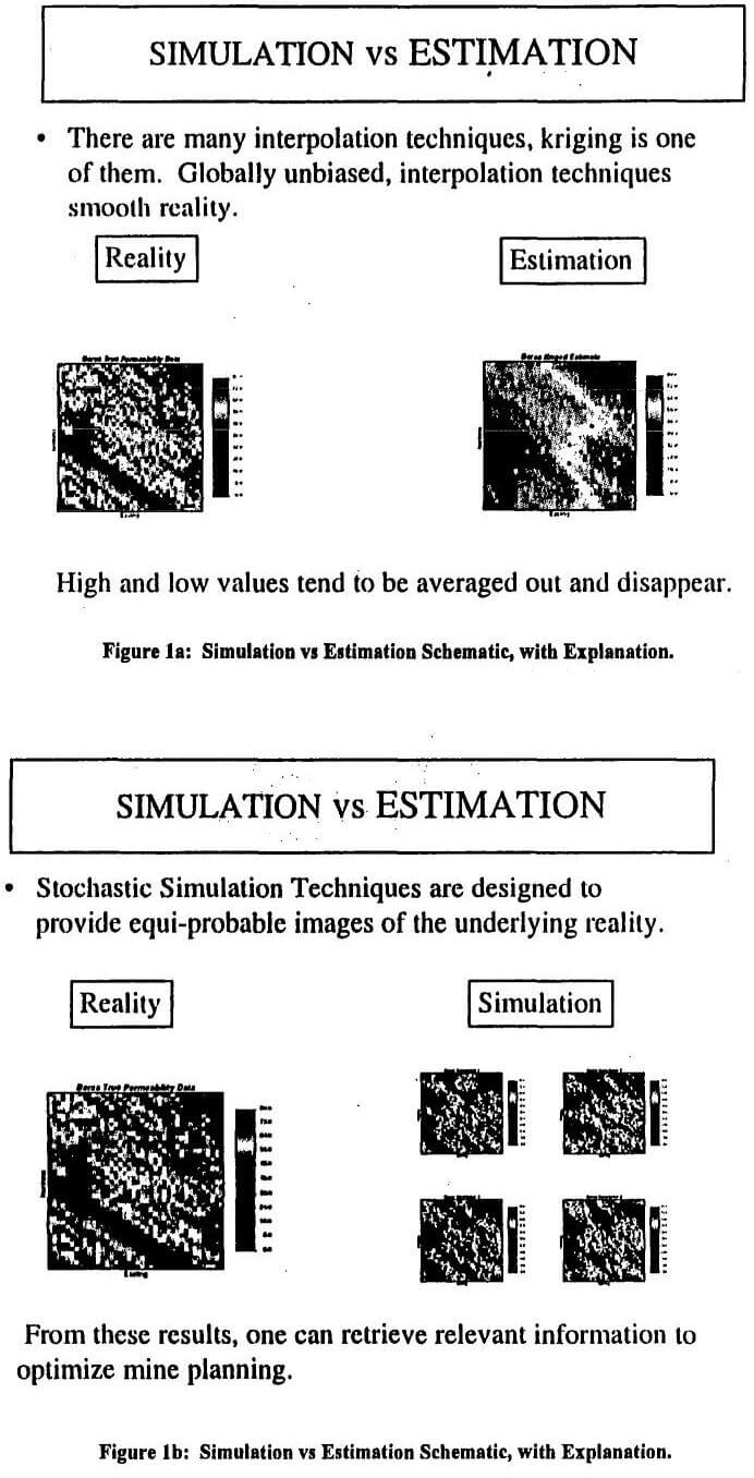
The idea is to build a number of block models that honor the histogram and the variogram of the original composite drill hole information. All conditional simulations are built on a fine grid, as fine as possible given the hardware available. Honoring the histogram means that the conditional simulation will correctly represent the proportion of high and low values, mean, variance, and other characteristics of the input drill hole data. Honoring the variogram means that reproduces the spatial complexity of the orebody, connectivity of high and low values, and the overall grade continuity in three dimensions. These characteristics of the deposits are all important pieces that can play a significant role when designing, planning, and scheduling an operation, see Figures 1a and 1b.

A number of issues have to be adequately resolved in practice for the simulations to be representative of the grades of the deposit. This includes, among other things, choosing among several simulation techniques available, such as Sequential Gaussian (Isaaks, 1990), Sequential Indicator (Alabert, 1987), or others. Also, decisions about grid sizes, conditioning data, search neighborhoods, treatment of high grade values, etc., must be made. It is a similar development process as when developing a kriging block model. More detailed discussions about practical implementations can be found in Deutsch and Journel (1992), and Rossi and Van Brunt (1997), among others.

When a number of these conditional simulations have been run and checked, then, for each block defined in the grid, there will be a corresponding number of different grades available in the model. These set of grades are interpreted to describe the model of uncertainty (Journel, 1988) for that block, generally arranged as a cumulative conditional probability curve.